Harmonic Analysis & Dynamic Modelling of VSI-Fed IM | Frequency-Controlled IM Drives

SECTION 01

Learning Outcomes

After this lecture you will be able to:

Derive the harmonic equivalent circuit of the IM and show that harmonic currents decay as \(I_n \propto 1/n^2\).
Compute the additional copper losses and THD introduced by six-step harmonic voltages.
Explain the rotating MMF directions of the 5th and 7th harmonics and predict the resulting torque-ripple frequency.
Write down Park's transformation matrix and the \(qdo\) voltage equations in the synchronous reference frame.
State the advantages of the synchronous frame model for controller design and harmonic analysis.
Set up the state-space model and periodic boundary condition for exact harmonic steady-state analysis of the VSI-fed IM.

SECTION 02

Harmonic Equivalent Circuit of the Induction Motor

Motor Response to Harmonic Voltages

For a harmonic of order \(n\), the rotor slip relative to the harmonic rotating field is:

\[s_n = \frac{n\omega_s \mp \omega_r}{n\omega_s} = \frac{n \mp 1}{n} \approx 1\]

The minus sign applies to positive-sequence harmonics (\(n = 6k+1\)) and the plus sign to negative-sequence harmonics (\(n = 6k-1\)). Since \(\omega_r \approx \omega_s\), \(s_n \approx 1\) for all significant harmonics.

Since \(s_n \approx 1\): the referred rotor impedance \(\approx R_r + jnX_{lr}\)
Magnetising reactance \(jnX_m \gg R_r\) → negligible harmonic air-gap flux
Harmonic currents flow mainly through total leakage reactance: \(X_{eq} = X_{ls} + X_{lr}\)

Harmonic current content for six-step VSI
\(n\)	\(I_n/I_1\)	Sequence
1	1.000	Positive
5	0.200	Negative
7	0.143	Positive
11	0.091	Negative
13	0.077	Positive

SECTION 03

Harmonic Current Decay Law

The \(1/n^2\) Decay Law

Harmonic current magnitude:

\[I_n \approx \frac{V_n}{n\,X_{eq}}, \qquad X_{eq} \approx X_{ls} + X_{lr}\]

Since the six-step VSI has \(V_n = V_1/n\) for all significant harmonics:

\[\boxed{I_n \approx \frac{V_1}{n^2\,X_{eq}} \quad \Rightarrow \quad I_n \propto \frac{1}{n^2}}\]

Higher-order harmonics decay very rapidly; the 5th and 7th dominate.

Voltage THD of the Six-Step Inverter

\[\mathrm{THD}_{V} = \frac{\sqrt{\sum_{n>1} V_n^2}}{V_1} = \sqrt{\sum_{n>1}\frac{1}{n^2}} \approx 28\%\]

Current THD is Lower than Voltage THD

Motor leakage inductance filters harmonics according to \(I_n/I_1 \propto 1/n^2\). Typical motor current \(\mathrm{THD}_I\): 15–25% (lower than \(\mathrm{THD}_V\); depends on \(X_{eq}\) and operating speed).

SECTION 04

Harmonic Losses & Torque Ripple in the Motor

Additional Motor Losses Due to Harmonics

\[\Delta P_{cu,s} = 3\sum_{n>1} I_n^2\,R_s \quad \text{(extra stator copper loss)}\]

\[\Delta P_{cu,r} = 3\sum_{n>1} I_n^2\,R_r \quad \text{(extra rotor copper loss, since } s_n\approx 1\text{)}\]

Additional core loss: eddy currents scale as \(n^2\); hysteresis loss as \(n\)
Total extra heating: approximately 10–25% → motor must be thermally derated
IEEE Std 112 recommends approximately 10% derating for six-step VSI-fed motors

Pulsating (Ripple) Torques

5th (negative seq.) + 7th (positive seq.) interact → torque ripple at \(6\omega_s\)
11th + 13th → torque ripple at \(12\omega_s\)
Consequences: audible noise, mechanical vibration, fatigue in gear teeth, reduced bearing life

Remedy: PWM

PWM techniques (Lecture 7E) shift harmonics to sideband frequencies around the carrier \(f_c\). Motor inductance filters them effectively → current is nearly sinusoidal → motor derating reduced from ~10% to ~1–3%.

SECTION 05

Harmonic Flux Linkages & Rotating MMF Directions

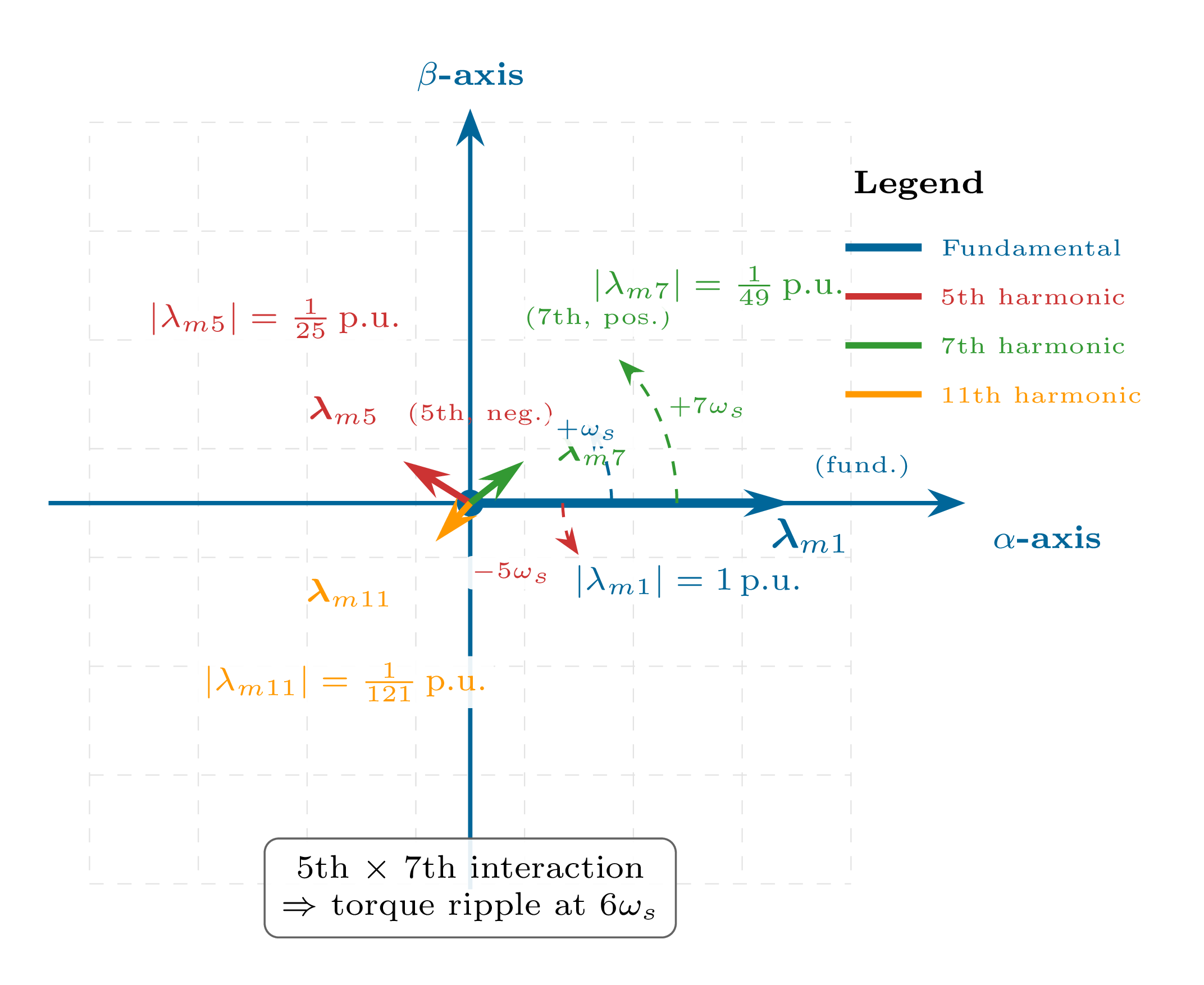
Rotating MMF Directions and Harmonic Slip

Harmonic flux linkage phasor diagram showing fundamental forward, 5th backward, and 7th forward rotating flux components — Harmonic flux linkage phasor diagram

Fundamental (\(n=1\)): Rotates at \(+\omega_s\) (forward direction)
5th (negative seq.): Rotates at \(-5\omega_s\) (backward). Slip \(s_5 \approx 6/5\). Produces backward air-gap flux and parasitic braking torque.
7th (positive seq.): Rotates at \(+7\omega_s\) (forward). Slip \(s_7 \approx 6/7\). Together with the 5th produces ripple at \(6\omega_s\).
11th + 13th: Produce torque ripple at \(12\omega_s\)

Harmonic MMF Sequence Rule (General)

\(n = 6k-1\): negative sequence (backward MMF)
\(n = 6k+1\): positive sequence (forward MMF), \(k = 1, 2, 3, \ldots\)

Memory aid: Alternates "−1, +1" around every multiple of 6.

Harmonic Rotor Flux Linkages

Flux linkage due to harmonic \(n\) decays as:

\[\lambda_{mn} \approx \frac{V_1/n}{n\,\omega_s\,L_{eq}}\cdot L_{lr} \quad \Rightarrow \quad \lambda_{mn} \propto \frac{1}{n^2}\]

Explicitly for the dominant 5th and 7th harmonics:

\[\lambda_{m5} \approx \frac{2V_{dc}}{25\pi\omega_s} \cdot \frac{L_{lr}}{L_{eq}}, \qquad \lambda_{m7} \approx \frac{2V_{dc}}{49\pi\omega_s} \cdot \frac{L_{lr}}{L_{eq}}\]

The rapid decay means harmonic flux (and thus harmonic torque) is much smaller than fundamental — the motor acts as a good low-pass filter for flux, but much less so for current.

SECTION 06

Park's Transformation & the Synchronous Reference Frame

Why Use a Reference Frame?

In the stationary (abc) frame: all voltages and currents are AC → PI controller design is complex because PI controllers cannot track AC references without steady-state error
Transforming to the synchronous (\(e\)) frame rotating at \(\omega_s\): fundamental quantities become DC in steady state
Enables straightforward PI controller design (no steady-state error for DC signals)
Zero-sequence (\(o\)) component is zero for balanced 3-phase — only \(q\) and \(d\) components needed
Provides the mathematical basis for Field-Oriented Control (FOC)

FOC Preview

In FOC: rotor flux is aligned with the \(d\)-axis: \(\lambda_{qr}^e = 0\), \(\lambda_{dr}^e = \lambda_r\)

\[T_e = \frac{3P}{4}\frac{L_m}{L_r}\,\lambda_r\,i_{qs}^e\]

\(\Rightarrow\) Torque \(= K \cdot \lambda_r \cdot i_{qs}^e\) — analogous to a separately excited DC motor. Covered in detail in Chapter 8.

Park's Transformation Matrix (abc → qd, amplitude-invariant)

\[\begin{bmatrix}f_q\\f_d\end{bmatrix} = \frac{2}{3} \begin{bmatrix} \cos\theta_e & \cos(\theta_e - 120°) & \cos(\theta_e + 120°)\\ -\sin\theta_e & -\sin(\theta_e - 120°) & -\sin(\theta_e + 120°) \end{bmatrix} \begin{bmatrix}f_a\\f_b\\f_c\end{bmatrix}\]

where \(\theta_e = \int \omega_s\,dt\) is the electrical angle of the synchronous frame. The transformation applies to any three-phase quantity \(f\) (voltage, current, or flux). In steady state, \(f_q\) and \(f_d\) are constant (DC), while harmonics appear as AC ripple superimposed on the DC values.

Advantages of the Synchronous Frame

Steady-state variables are DC → PI controllers achieve zero steady-state error
Basis for FOC: orient \(d\)-axis along rotor flux → \(i_{ds}^e\) controls flux; \(i_{qs}^e\) controls torque
Same equations used for small-signal linearisation and stability analysis
Harmonics appear as AC ripple on DC values — easily identified and filtered

SECTION 07

QDO Voltage Equations & Electromagnetic Torque

Complete \(qdo\) Voltage Matrix in the Synchronous Frame

\[\begin{bmatrix}v^e_{qs}\\v^e_{ds}\\0\\0\end{bmatrix} = \begin{bmatrix} R_s + L_s p & \omega_s L_s & L_m p & \omega_s L_m\\ -\omega_s L_s & R_s + L_s p & -\omega_s L_m & L_m p\\ L_m p & \omega_{sl} L_m & R_r + L_r p & \omega_{sl} L_r\\ -\omega_{sl} L_m & L_m p & -\omega_{sl} L_r & R_r + L_r p \end{bmatrix} \begin{bmatrix}i^e_{qs}\\i^e_{ds}\\i^e_{qr}\\i^e_{dr}\end{bmatrix}\]

where \(p = d/dt\), \(L_s = L_{ls} + L_m\), \(L_r = L_{lr} + L_m\), and \(\omega_{sl} = \omega_s - \omega_r\) is the slip angular frequency. The superscript \(e\) denotes synchronous frame quantities.

Electromagnetic Torque

\[T_e = \frac{3}{2} \cdot \frac{P}{2} \cdot L_m \left(i^e_{qs}\,i^e_{dr} - i^e_{ds}\,i^e_{qr}\right)\]

Mechanical Equation

\[J\,\frac{d\omega_r}{dt} = T_e - T_l - B\omega_r\]

\(\omega_r\) = rotor mechanical speed (rad/s), \(J\) = rotor inertia (kg·m²), \(B\) = viscous friction (N·m·s/rad), \(T_l\) = load torque (N·m).

SECTION 08

State-Space Model & Periodic Steady-State Solution

State-Space Form of the \(qdo\) Equations

The \(qdo\) equations can be written in the standard state-space form:

\[\dot{\mathbf{x}} = \mathbf{A}\,\mathbf{x} + \mathbf{B}\,\mathbf{u}, \qquad \mathbf{x} = \begin{bmatrix} i^e_{qs} & i^e_{ds} & i^e_{qr} & i^e_{dr} \end{bmatrix}^\top\]

Six-step VSI applies periodic switching at \(T_s/6\) intervals
Voltage vector \(\mathbf{u}\) is piecewise-constant in each 60° interval
Exact solution within interval \(k\) via the matrix exponential:

\[\mathbf{x}(t) = e^{\mathbf{A}t}\,\mathbf{x}(0) + \mathbf{A}^{-1}\!\left(e^{\mathbf{A}t} - \mathbf{I}\right)\mathbf{B}\,\mathbf{u}\]

Periodic Boundary Condition

Due to the 3-phase symmetry of the six-step pattern, the state at the end of each 60° interval is a rotated version of the state at the beginning:

\[\mathbf{x}\!\left(\frac{\pi}{3\omega_s}\right) = S_1\,\mathbf{x}(0)\]

where \(S_1\) is the \(60°\) rotation (transition) matrix. Solving for \(\mathbf{x}(0)\) yields the exact periodic steady state in one linear solve.

Transition Matrix \(S_1\) and Computational Advantage

60° Boundary Rotation Matrix \(S_1\)

\[S_1 = \begin{bmatrix} \tfrac{1}{2} & \tfrac{\sqrt{3}}{2} & 0 & 0\\ -\tfrac{\sqrt{3}}{2} & \tfrac{1}{2} & 0 & 0\\ 0 & 0 & \tfrac{1}{2} & \tfrac{\sqrt{3}}{2}\\ 0 & 0 & -\tfrac{\sqrt{3}}{2} & \tfrac{1}{2} \end{bmatrix}\]

Each 60° switching advance rotates both the stator and rotor current vectors by \(-60°\) in the synchronous frame. The block-diagonal structure reflects the decoupled \(q\)- and \(d\)-axis pairs.

What the Periodic Steady-State Solution Provides

Phase currents \(i_{as}(t)\): full waveform including all harmonic content
Instantaneous and average electromagnetic torque
RMS currents, harmonic copper losses, and efficiency
Torque ripple magnitudes at \(6\omega_s\) and \(12\omega_s\)
Input displacement power factor

Computational advantage: True periodic steady state (all harmonic effects) obtained in a single matrix inversion — orders of magnitude faster than transient time-domain simulation.