PWM Strategies & Harmonic Control

After this lecture you will be able to:

Explain why PWM shifts low-order harmonics to sideband frequencies and how motor inductance filters them.
Calculate the fundamental output voltage of an SPWM inverter given modulation index \(m_a\) and DC bus voltage \(V_{dc}\).
Describe third-harmonic injection and quantify its DC-bus utilisation improvement over basic SPWM.
State the SHE transcendental equations for eliminating the 5th and 7th harmonics and describe how they are solved.
Draw the SVM hexagon, label all eight voltage vectors, and compute dwell times \(T_1\), \(T_2\), \(T_0\) for a given reference.
Compare SPWM, SHE, and SVM on THD, DC utilisation, switching loss, and implementation complexity.

Problems with Six-Step VSI and the PWM Solution

Harmonic spectra comparison: six-step VSI with large 5th and 7th harmonics versus SPWM showing harmonics shifted to sideband frequencies around carrier — Harmonic spectra: six-step vs. SPWM (\(m_f = 19\)); low-order harmonics eliminated and shifted to sideband frequencies

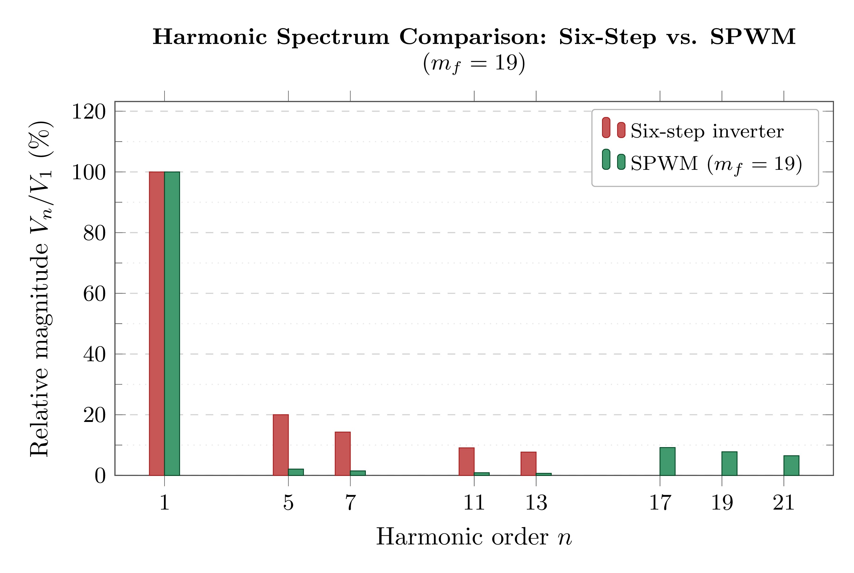
Problems with Six-Step VSI:

Large 5th and 7th harmonic voltages (20% and 14% of fundamental)
Motor heating, derating (~10%), and audible noise
Torque ripple at \(6\omega_s\) — problematic in precision drives
\(\mathrm{THD}_V \approx 28\%\); IEEE 519 line limit is 5%

PWM Principle:

Vary pulse widths so the fundamental is preserved but harmonics are pushed to much higher frequencies
Motor leakage inductance naturally filters high-frequency harmonics → near-sinusoidal current
Key trade-off: higher \(f_{sw}\) → better harmonics but more switching losses and EMI

Sideband Harmonic Locations for SPWM

Harmonics appear at: \((m_f \pm 2)f_s\), \((2m_f \pm 1)f_s\), \((3m_f \pm 2)f_s\), etc. Motor inductance filters these effectively at \(f_c \gt 1\) kHz, yielding smooth, near-sinusoidal current.

Four Main PWM Methods

SPWM — Sinusoidal PWM: Simplest and most common; compares sine reference with triangular carrier
SPWM+3H — SPWM with Third-Harmonic Injection: Extends the linear modulation range; improves DC utilisation to 90.7%
SHE — Selected Harmonic Elimination: Pre-computed switching angles that analytically eliminate specific harmonics; offline computation, lookup table in real time
SVM — Space Vector Modulation: Uses the voltage space vector hexagon concept; highest DC utilisation (90.7%); most common in DSP-based drives

SPWM Operating Principle

SPWM waveforms showing sinusoidal reference voltage versus triangular carrier (top) and resulting PWM pole voltage Va0 (bottom) — SPWM: sinusoidal reference vs. triangular carrier (top) and resulting PWM pole voltage \(v_{a0}\) (bottom)

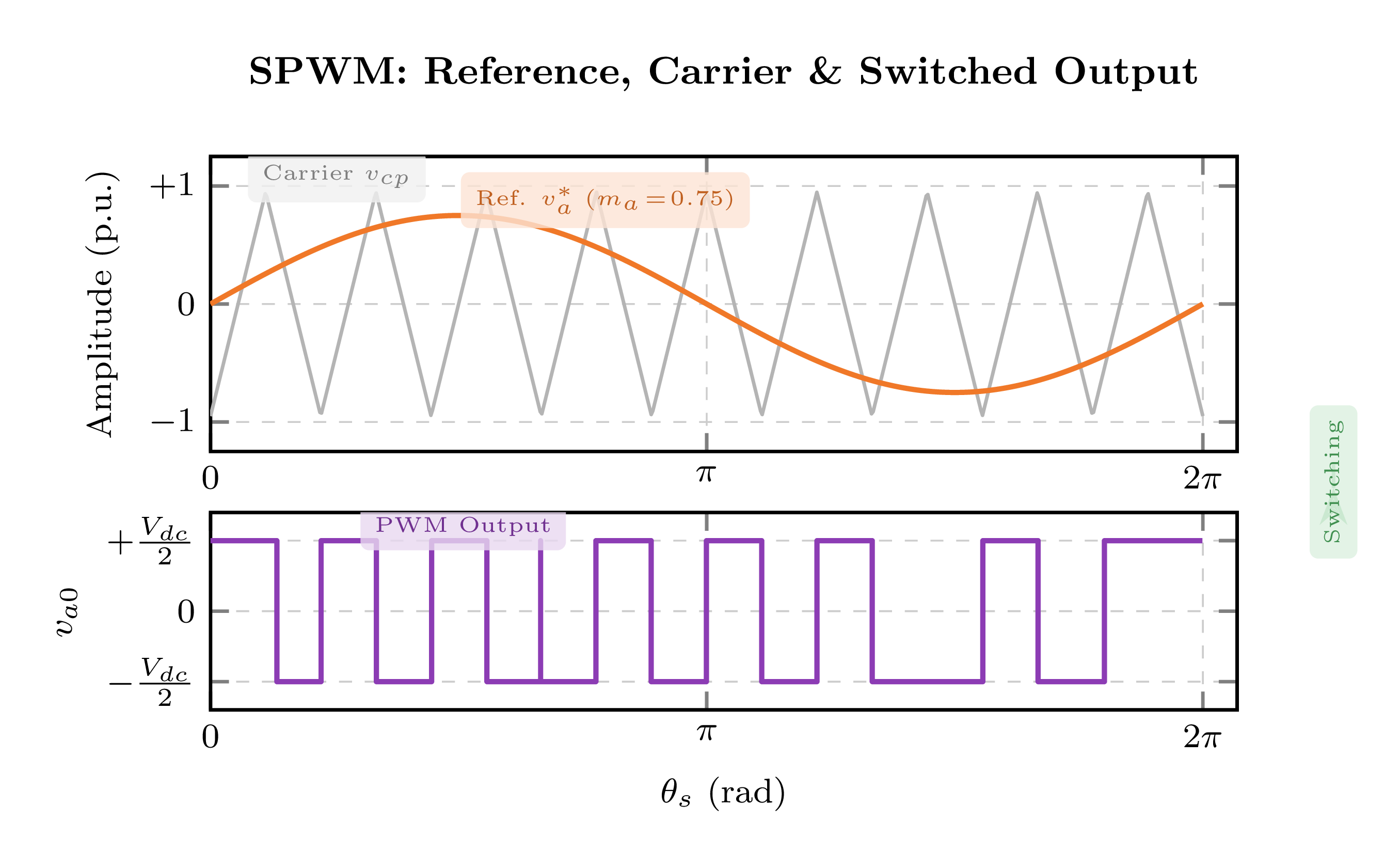
Reference: sinusoidal \(v_a^*(t) = m_a\,\hat{V}_{cp}\sin(\omega_s t)\)
Carrier: triangular waveform at \(f_c = m_f \cdot f_s\)
\(v_a^* > v_{cp}\): upper IGBT ON (\(+V_{dc}/2\))
\(v_a^* < v_{cp}\): lower IGBT ON (\(-V_{dc}/2\))
Pulse widths vary sinusoidally → fundamental preserved

SPWM Key Parameters

Modulation index: \(m_a = \hat{v}_a^*/\hat{v}_{cp}\), \(\;0 \leq m_a \leq 1\)

Frequency ratio: \(m_f = f_c/f_s\) (odd integer preferred)

Output fundamental (pole voltage peak):

\[\hat{V}_{a0,1} = m_a \cdot \frac{V_{dc}}{2} \quad (m_a \leq 1)\]

Linear range: \(0 \leq m_a \leq 1\); DC bus utilisation: 78.5%

Rules for Best SPWM Performance

\(m_f\) should be an odd integer — avoids even-order harmonics (ensures half-wave symmetry)
\(m_f\) should be a multiple of 3 — triplen harmonics in pole voltage cancel in line voltages
Recommended values: \(m_f = 9,\;15,\;21,\;\ldots\) (odd multiples of 3)
Above \(m_f \approx 9\), the harmonic performance is nearly independent of \(m_f\) — the dominant factor becomes \(m_a\)

Concept: Extending the Linear Range of SPWM

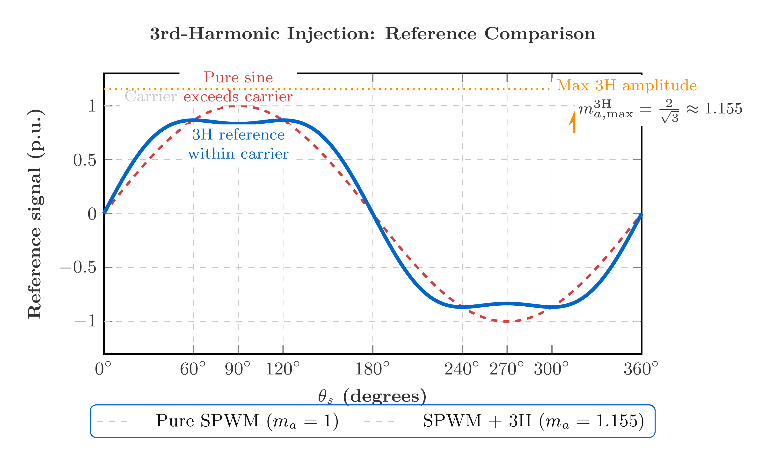
Reference signal comparison: pure sinusoid reaching carrier peak versus sinusoid with third-harmonic injection staying within carrier envelope at higher fundamental amplitude — Reference signal: pure sine vs. sine + third-harmonic injection; the 3H reference stays within the carrier envelope while extending the linear range

In a balanced 3-phase system, a third-harmonic component in the reference is common-mode: it appears identically in all three phase references
Common-mode voltage does not appear in line-to-line voltages (it cancels by subtraction)
Adding a 3rd harmonic term allows phase references to exceed the carrier peak before line voltages become distorted → linear range is extended

Third-Harmonic Injection Reference Signal

\[v_a^*(t) = m_a\hat{V}_{cp}\!\left[\sin(\omega_s t) + \frac{1}{6}\sin(3\omega_s t)\right]\]

The optimum injection ratio is 1/6 (equivalently \(\frac{1}{2\sqrt{3}} \approx 0.289\)). This is the value that maximally flattens the reference peak and gives the greatest extension of the linear range.

Performance Improvement with Third-Harmonic Injection

Maximum Linear Modulation Index

\[m_{a,max} = \frac{2}{\sqrt{3}} \approx 1.155\]

This is a 15.5% increase over the SPWM maximum of 1.0, directly translating into higher output voltage for the same DC bus.

DC Bus Utilisation: 90.7%

This equals the SVM utilisation, making SPWM+3H equivalent to SVM in the linear modulation range. SPWM+3H is simpler to implement in analog hardware, while SVM is more natural for DSP-based digital control.

SPWM vs. SPWM+3H performance comparison
Feature	SPWM	SPWM+3H
Max. linear \(m_a\)	1.000	1.155
DC bus utilisation	78.5%	90.7%
Line voltage THD	~10%	~8%
Complexity	Low	Low+
Equivalent to	—	SVM (in linear range)

SHE Principle: Pre-Computed Switching Angles

SHE selects switching angles in advance to simultaneously control the fundamental voltage amplitude and analytically cancel selected low-order harmonics. For a quarter-wave symmetric waveform with \(N\) switching angles \(\alpha_1 < \alpha_2 < \cdots < \alpha_N\) in the range \(0° < \alpha_i < 90°\), the Fourier coefficients of the \(n\)th harmonic can be made zero.

Typical design goal: Eliminate 5th and 7th harmonics with 3 switching angles per quarter period:

\[\cos(\alpha_1) - \cos(\alpha_2) + \cos(\alpha_3) = \frac{\pi}{4}\,m_a\]

\[\cos(5\alpha_1) - \cos(5\alpha_2) + \cos(5\alpha_3) = 0\]

\[\cos(7\alpha_1) - \cos(7\alpha_2) + \cos(7\alpha_3) = 0\]

These are three transcendental equations in three unknowns. They have no closed-form solution and are solved numerically (e.g., Newton-Raphson) for each desired \(m_a\). The angle sets are pre-computed and stored in lookup tables indexed by \(m_a\).

SHE Advantages

Analytically eliminates specified low-order harmonics (5th, 7th, 11th, etc.)
Achieves very low line-voltage THD (<5%) with minimal switching events
Lower switching frequency than SPWM → reduced switching losses
Preferred for GTO/IGCT-based high-power drives where switching loss is critical

SHE Limitations

Offline computation required; angles stored as lookup tables indexed by \(m_a\)
Dynamic response limited by lookup table update rate
DC bus utilisation limited to 78.5% (same as basic SPWM without 3H injection)
Cannot directly extend to overmodulation as easily as SVM

Concept: Voltage Space Vectors

SVM voltage hexagon showing six active vectors V1 through V6 at 60-degree intervals, two zero vectors V0 and V7, reference vector V* in Sector 1, and inscribed SPWM circle — SVM hexagon: six active vectors \(V_1\)–\(V_6\), two zero vectors \(V_0/V_7\), reference \(\mathbf{V}^*\) in Sector 1, and the SPWM inscribed circle

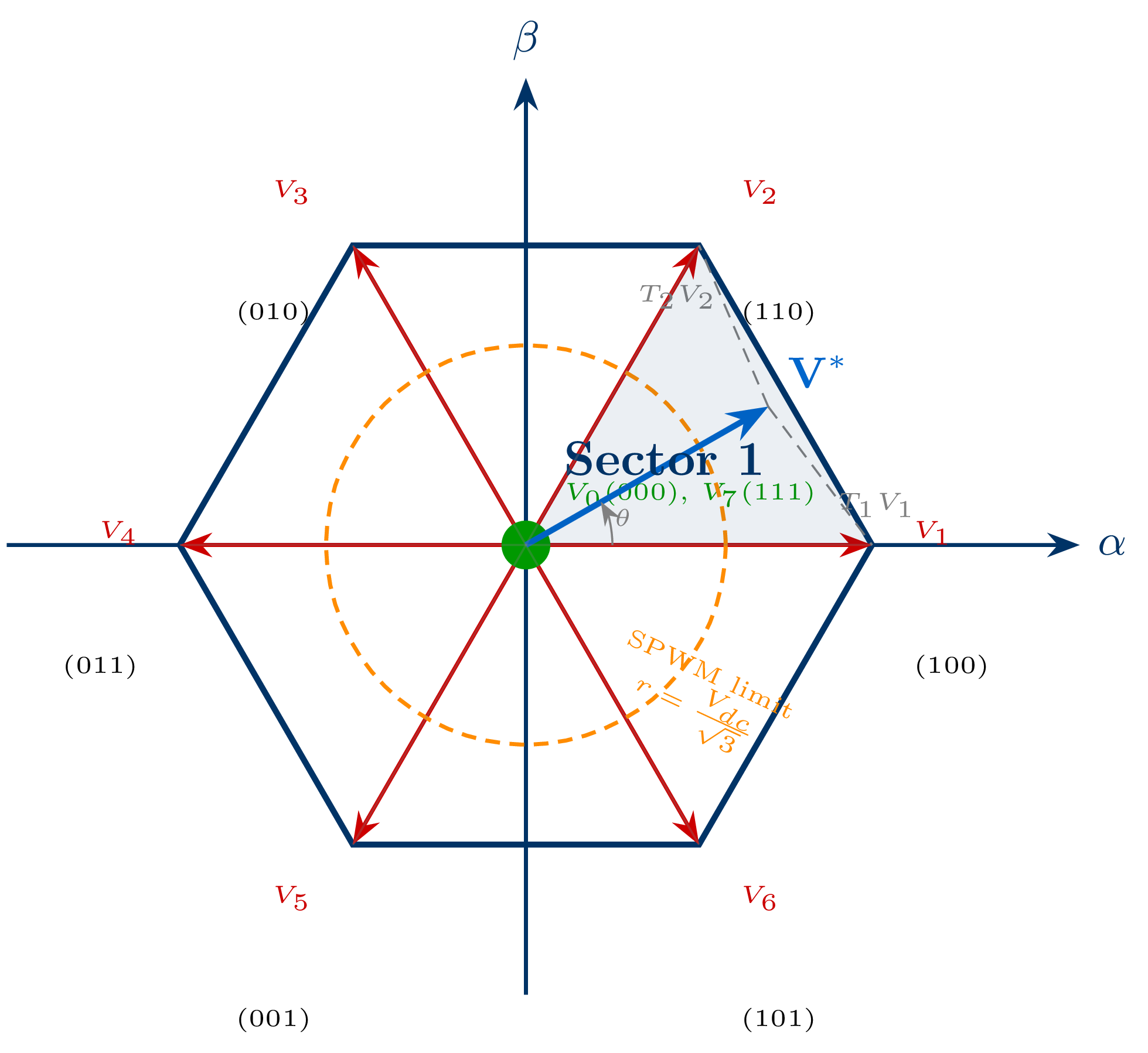
Three-phase VSI has \(2^3 = 8\) possible switch states
6 active vectors (\(V_1\)–\(V_6\)) at 60° intervals in the \(\alpha\beta\) complex plane
2 zero vectors (\(V_0\) = 000, \(V_7\) = 111): output voltage = 0
Reference \(\mathbf{V}^*\) synthesised by time-averaging adjacent active vectors plus zero vectors within each switching period \(T_s\)

Dwell-Time Equations (Sector 1, \(0° \leq \theta < 60°\))

\[T_1 = T_s \cdot m_a \cdot \sin(60° - \theta)\]

\[T_2 = T_s \cdot m_a \cdot \sin\theta\]

\[T_0 = T_7 = \frac{T_s - T_1 - T_2}{2}\]

where \(m_a\) is the SVM modulation index (normalised reference magnitude) and \(\theta\) is the angle of \(\mathbf{V}^*\) within the sector.

SVM Linear Modulation Limit and DC Bus Utilisation

Maximum Linear Modulation Index

\[m_{a,max}^{SVM} = \frac{1}{\sqrt{3}} \approx 0.577 \quad (\text{normalised to } V_{dc}/2)\]

Alternatively expressed as: the maximum length of \(\mathbf{V}^*\) that remains inside the hexagon is \(V_{dc}/\sqrt{3}\), corresponding to 90.7% of the maximum six-step fundamental \(2V_{dc}/\pi \cdot (\pi/2\sqrt{3}) = V_{dc}/\sqrt{3}\).

SVM vs. SPWM Advantages

15% higher DC bus voltage utilisation (90.7% vs. 78.5%)
Lower current THD for same switching frequency
Fewer switch transitions per cycle (optimised zero-vector placement)
Natural for DSP/FPGA implementation using look-up tables or direct computation
Seamless extension to field-oriented control
Mathematically equivalent to SPWM with optimum 3H injection

All PWM Methods at a Glance

Comprehensive comparison of PWM strategies for VSI-fed induction motor drives
Method	Low-Order Harmonics	Bus Utilisation	THD (line V)	Switching Loss
Six-step	High (20%, 14%)	78.5%	28%	Very low
SPWM	Moved to sidebands	78.5%	~10%	Medium
SPWM+3H	Moved to sidebands	90.7%	~8%	Medium
SHE	Analytically eliminated	78.5%	<5%	Low
SVM	Moved to sidebands	90.7%	~8%	Medium

Practical Selection Guide

Low power (<15 kW): SPWM is standard; simplest to implement
General industrial drives: SVM preferred — best DC utilisation, DSP-friendly, integrates with FOC
High power (GTO/IGCT-based): SHE — minimal switching loss; offline angle computation acceptable
Medium-voltage drives (>2 MW): Multi-level converters (NPC, flying capacitor, cascaded H-bridge)

Multi-Level Inverters for Medium Voltage

For >2 MW or medium-voltage applications, NPC (Neutral Point Clamped), flying capacitor, and cascaded H-bridge topologies offer much better harmonic performance and reduced \(dv/dt\) stress on motor windings. Each device blocks only \(V_{dc}/(N-1)\), enabling higher voltage operation with standard voltage-rated IGBTs.

Synchronised vs. Free-Running Carrier

Carrier frequency scheduling diagram showing stepped synchronised carrier at low output frequencies transitioning to fixed carrier frequency above 40 Hz crossover — Carrier frequency scheduling: synchronised (stepped) at low \(f_s\) and fixed above 40 Hz

Low output frequencies (\(f_s < 40\) Hz):

Carrier synchronised to output (\(m_f\) = odd integer, multiple of 3)
Prevents sub-harmonic torque ripple that would otherwise cause unacceptable noise and vibration
As \(f_s\) increases, \(m_f\) is stepped down in discrete jumps (e.g., 27, 21, 15, 9)

High output frequencies (\(f_s > 40\) Hz):

Carrier fixed at \(f_c \approx 4\)–10 kHz (free-running, asynchronous)
Harmonic performance is acceptable because \(m_f\) remains large enough
Smooth transition at the crossover frequency (\(\approx 40\) Hz)

Learning Outcomes

Motivation: From Six-Step to PWM

Sinusoidal Pulse-Width Modulation (SPWM)

Third-Harmonic Injection (SPWM + 3H)

Selected Harmonic Elimination (SHE) PWM

Space Vector Modulation (SVM)

PWM Method Comparison

Carrier Frequency Scheduling