Learning Outcomes
- Express the ASCI stator currents in the synchronous \(qd\) frame as piecewise functions of \(I_{dc}\) and \(\theta_s\).
- Write the plant differential equations of the closed-loop ASCI drive and identify the role of each state variable.
- State the controller equations and explain the minimum-copper-loss current command strategy.
- Describe the structural advantages of the PWM-CSI over the ASCI (no commutation capacitors, lower THD, no voltage spikes).
- Select the appropriate drive type (VSI, CSI, or cycloconverter) given application requirements of power, speed, and regeneration.
- Recall the key equations of the chapter and apply them to a given drive specification.
Steady-State Model: ASCI-Fed IM in the Synchronous QD Frame
Piecewise Representation
The ASCI produces piecewise-constant stator line currents (quasi-square waveform). After applying Park's transformation to the synchronous \(qd^e\) frame (rotating at \(\omega_s\)), the stator currents within each 60° switching interval \(k\) are expressed as:
where the trigonometric coefficients within interval \(k\) are:
\(\theta_s = \omega_s t\) is the synchronous frame angle; \(k = 1, 2, \ldots, 6\) indexes the six 60° intervals per fundamental cycle.
Physical Interpretation
In the synchronous frame, the fundamental component of the stator current appears as a DC vector, while the harmonic components (5th, 7th, 11th, …) appear as AC ripple at 6th, 12th, … multiples of \(\omega_s\). The piecewise-constant functions \(g_c\) and \(g_s\) capture this behaviour exactly within each interval.
60° Boundary Rotation Matrix
Rotation Matrix \(S_1\)
At each 60° switching boundary, the next gating event advances the stator current vector by 60° in the ABC frame. In the synchronous \(qd\) frame — which is itself rotating at \(\omega_s\) — this switching event appears as a rotation of the current vector by \(-60°\) (clockwise). This is captured by the matrix \(S_1\):
Unified Periodic Boundary Approach
This is the same \(S_1\) rotation matrix that appears in the VSI harmonic analysis (Lecture 7D), where it described the 60° rotation of the stator voltage vector at each switching event. The identical mathematical structure confirms that both the VSI (voltage-source) and the CSI (current-source) periodic steady states can be computed by the same technique: set up the state-space equations in each 60° interval and apply the periodic boundary condition \(\mathbf{x}(T_s) = \mathbf{x}(0)\), solved as a single matrix inversion.
Rotor Flux Equations in the Synchronous Frame
Rotor Voltage Equations (Referred to Stator)
The rotor is short-circuited; its voltage equations in the synchronous frame are:
\(\omega_{sl} = \omega_s - \omega_r\) is the slip angular frequency.
Rotor Flux Linkage Definitions
\(L_r = L_{lr} + L_m\) = total rotor self-inductance (per phase, referred to stator); \(L_m\) = magnetising inductance; \(i_{qs}^e\), \(i_{ds}^e\) = stator current components (input, treated as known from \(g_c\,I_{dc}\) and \(g_s\,I_{dc}\)).
Electromagnetic Torque
This is the general cross-product torque expression valid in any reference frame. With rotor-flux orientation (\(\lambda_{qr}^e = 0\)), it simplifies to the familiar FOC expression \(T_e = (3P/4)(L_m/L_r)\,\lambda_{dr}^e\,i_{qs}^e\).
Voltage Spike at Commutation
Origin of the Spike
During commutation, the stator current changes abruptly from one phase pair to another. This rapid \(di/dt\) through the stator transient leakage inductance \(L_s' = L_s - L_m^2/L_r\) generates an impulsive voltage spike at the motor terminals:
\(L_s'\) = stator transient (subtransient) leakage inductance = \(L_s - L_m^2/L_r\); \(\Delta I_{dc}\) = step change in stator current during commutation; \(\Delta t_{comm}\) = commutation time (determined by the commutation capacitor and \(L_s'\)).
Consequences:
- Peak motor terminal voltage can be 1.5–2× the fundamental peak value
- Motor winding insulation must be rated accordingly
- Increases insulation ageing and reduces motor lifespan if not managed
Mitigation Measures:
- Connect snubber capacitors (5–20 μF) directly across motor terminals — these absorb the impulsive energy and limit \(dv/dt\)
- Select motors with reinforced turn-to-turn insulation when used with CSI drives
- Use a PWM-CSI instead of ASCI — this eliminates the step-change in current and hence the spike
Dynamic Model: State Variables
State Vector
| State | Symbol | Physical Quantity |
|---|---|---|
| \(x_1\) | \(I_{dc}\) | DC link current (A) — the controlled current source |
| \(x_2\) | \(\lambda_{qr}^e\) | \(q\)-axis rotor flux linkage in sync. frame (Wb) |
| \(x_3\) | \(\lambda_{dr}^e\) | \(d\)-axis rotor flux linkage in sync. frame (Wb) |
| \(x_4\) | \(\omega_r\) | Rotor mechanical speed (rad/s) |
| \(x_5\) | \(\varepsilon_\omega\) | Speed PI controller integrator state |
| \(x_6\) | \(\varepsilon_I\) | DC current PI controller integrator state |
Plant Differential Equations
DC Link Current Dynamics
The factor \(2L_s'\) appears because, at any instant, two stator phases are conducting in series through the DC link. \(v_r\) is the rectifier output voltage (the control input).
Rotor Flux Dynamics
These equations describe the first-order lag of the rotor flux linkages. The rotor time constant is \(\tau_r = L_r/R_r\); large rotors have a long time constant and slow flux dynamics.
Mechanical Dynamics
Newton's second law for the rotating mass: \(J\) = rotor inertia (kg·m²); \(B\) = viscous friction coefficient (N·m·s/rad); \(T_l\) = load torque. The electromagnetic torque term \(\frac{3L_m}{2L_r}(g_c\,x_3 - g_s\,x_2)\,x_1\) is the cross-product of the current and flux vectors.
Anti-Windup Limiters
- Rectifier voltage limit: \(|v_r^*| \le V_{cm}\) — prevents rectifier saturation
- Slip speed limiter: \(|\omega_{sl}^*| \le \omega_{sl,max} = R_r/L_{lr}\) — prevents operation beyond the breakdown torque point and motor stalling
Together, these limits ensure stable operation during large load transients and speed reversal manoeuvres.
Controller Equations
Outer Speed Loop — Slip-Speed Command
\(K_{ps}\) and \(K_{is}\) are the proportional and integral gains of the outer speed PI controller. \(\dot{x}_5 = \omega_r^* - \omega_r\) is the speed error; \(x_5\) is the integral of the speed error.
Stator Frequency Command
The stator (inverter) frequency is synthesised by adding the measured rotor speed \(x_4 = \omega_r\) to the commanded slip speed \(\omega_{sl}^*\). This is the fundamental frequency-synthesis equation used in all scalar drives.
DC Current Command — Minimum Copper Loss
\(K_{tg} = \frac{3P}{4}\frac{L_m^2}{L_r}\,I_m\) is the torque gain constant (N·m/A); \(I_m\) is the rated magnetising current. This expression selects the DC link current that minimises total stator plus rotor copper losses at the current operating slip. At light load (\(\omega_{sl}^*\) small), \(I_{dc}^*\) is reduced below its rated value, lowering flux and losses.
Inner Current Loop — Rectifier Voltage Command
\(K_{pi}\) and \(K_{ii}\) are the proportional and integral gains of the inner current PI controller. \(\dot{x}_6 = I_{dc}^* - I_{dc}\) is the current error. The output \(v_r^*\) is converted to the rectifier firing angle \(\alpha = \cos^{-1}(v_r^*/V_{r,max})\).
Cascade Stability Criterion
For stable cascaded control, the inner loop (current) must have a bandwidth 5–10× higher than the outer loop (speed). Typical values: inner loop bandwidth 50–200 Hz; outer speed loop 5–20 Hz. This separation of timescales allows each loop to be designed and tuned independently.
PWM Current-Source Inverter Drive
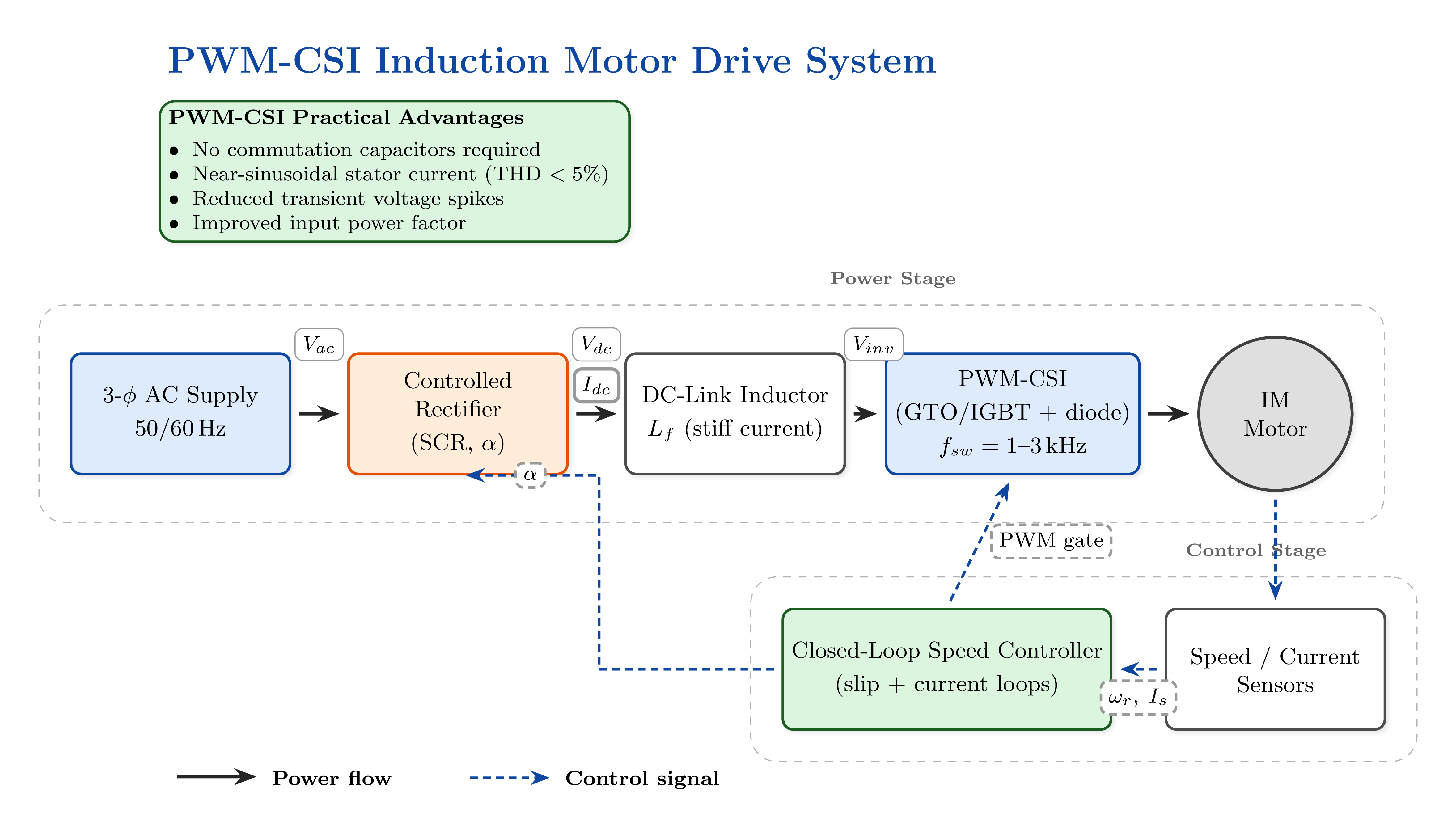
Key Structural Changes from ASCI
- Replace SCRs with GTOs or IGBTs (self-commutating devices): no commutation capacitors are required
- Each IGBT must have a series diode to block reverse current through the IGBT's built-in body diode — this preserves the unidirectional (current-source) DC-link characteristic
- Small output filter capacitors (connected line-to-line at motor terminals) are needed to provide a path for the commutation current during PWM switching and to limit \(dv/dt\) at motor terminals
- PWM algorithms (sinusoidal PWM or SVM applied to current references) shape the output current to be near-sinusoidal
IGBT Body Diode Problem
Unlike a VSI, the CSI's DC link carries a unidirectional current (\(I_{dc} > 0\) always). The IGBT's anti-parallel body diode would allow reverse current to flow through the switch arm during the OFF state, which would short-circuit the DC link inductor and destroy the current-source behaviour. Adding a series diode in each arm blocks this reverse-current path, so the DC-link current can only flow through the IGBT when it is gated ON.
Output Filter Capacitors
When an IGBT turns OFF in the PWM-CSI, the DC-link current (\(I_{dc}\)) must continue to flow — there is no freewheeling path through the motor phases. Small capacitors connected across the motor terminals (typically 5–30 μF per phase) provide this momentary path, absorbing the \(I_{dc}\) pulse and limiting the resulting \(dv/dt\). They also reduce the voltage spikes that were a concern with the ASCI.
ASCI vs. PWM-CSI: Comparison
| Feature | ASCI | PWM-CSI |
|---|---|---|
| Switching device | SCR (thyristor) | GTO or IGBT + series diode |
| Turn-off method | Commutation capacitor | Gate signal (self-commutated) |
| Commutation capacitors | Required (3 large capacitors) | None |
| Output filter capacitors | Optional (snubbers) | Required (small, 5–30 μF) |
| Switching frequency | \(< 500\) Hz | 1–3 kHz |
| Output current waveform | Quasi-square (120°) | Near-sinusoidal |
| Current THD | ~31% | <5% |
| Motor voltage spikes | Present (insulation stress) | Eliminated |
| Motor derating | 10–15% | 1–3% |
| Regeneration | Yes (natural) | Yes (natural) |
| Cost | Lower (SCRs cheap) | Higher (GTO/IGBT + diodes) |
| Typical power range | 100 kW – several MW | 500 kW – 10 MW |
Typical Applications of PWM-CSI
- High-power fans, pumps, and compressors (500 kW – 10 MW)
- Ship propulsion systems requiring smooth, low-noise operation
- Rolling mills and mine hoists requiring regenerative braking
- Applications where standard motors (not reinforced insulation) must be used
- For drives above 10 MW, the Load-Commutated Inverter (LCI) with synchronous motors is an alternative
Chapter Summary
| Lecture | Title | Key Topics |
|---|---|---|
| 7A | Introduction & Static Frequency Changers | Synchronous speed, affinity laws, cycloconverter, matrix converter, VSI vs. CSI overview |
| 7B | Voltage-Source Inverter: Circuit & Operation | McMurray circuit, IGBT bridge, six-step gating, pole/line/phase voltages, harmonic spectrum |
| 7C | VSI-Fed IM: Steady State & V/f Control | Per-phase equivalent circuit, constant V/f, IR-boost, slip-speed control, constant air-gap flux |
| 7D | Harmonic Analysis & Dynamic Modelling | Harmonic circuit, \(1/n^2\) decay, torque ripple, Park's transform, \(qdo\) equations, periodic steady state |
| 7E | PWM Strategies & Harmonic Control | SPWM, 3H-injection, SHE, SVM (hexagon, dwell times), carrier scheduling, method comparison |
| 7F | Current-Source Inverter: ASCI Drive | DC-link inductor, ASCI commutation (4 stages), quasi-square current, torque, regeneration, closed-loop control |
| 7G | CSI Dynamics, PWM-CSI & Chapter Summary | QD-frame ASCI model, state variables, plant ODEs, controller equations, PWM-CSI, drive selection |
| Strategy | Feedback | Speed Accuracy | Best Application |
|---|---|---|---|
| Constant V/Hz | None | ±2–5% | Fans, pumps, compressors — low cost |
| Constant slip speed | Speed sensor | <1% | General-purpose conveyors, machine tools |
| Constant air-gap flux | \(V_s\), \(I_s\) sensors | <0.5% | High-performance drives, good low-speed torque |
Limitation of All Scalar Methods
All V/f strategies control only the magnitude of voltage (or flux) — flux and torque cannot be independently controlled. The dynamic torque-step response is slow (typically >50 ms). For fast dynamics, Field-Oriented Control (FOC) or Direct Torque Control (DTC) are required (Chapter 8).
| Method | Low-Order Harmonics | DC Bus Utilisation | THD | Switching Loss |
|---|---|---|---|---|
| Six-step (180°) | High (5th, 7th dominant) | 78.5% | 28% | Very low |
| SPWM | Shifted to sidebands | 78.5% | ~10% | Medium |
| SPWM + 3H injection | Shifted to sidebands | 90.7% | ~8% | Medium |
| SHE PWM | Eliminated by design | 78.5% | <5% | Low |
| SVM | Shifted to sidebands | 90.7% | ~8% | Medium |
Drive Selection Guide
| Application | Recommended Drive Type | Reason |
|---|---|---|
| Fan/pump (<2 MW) | Diode rectifier + PWM-VSI | Low cost, unidirectional, simple V/f control sufficient |
| High-speed precision (CNC) | SVM-VSI + FOC | Best dynamic response; near-sinusoidal currents |
| Regenerative elevator/hoist | AFE-VSI (active front-end) | Returns braking energy to grid; high PF; no braking resistor |
| Very low speed (<10 Hz) gearless | Cycloconverter | Direct AC–AC; \(f_{out}\) limited to \(\frac{1}{3}f_{in}\); high power; ball mills |
| High-power regenerative (100 kW – MW) | CSI (ASCI or PWM-CSI) | Natural four-quadrant operation; frequency-independent \(T_{max}\) |
| Medium voltage (>2 MW) | Multi-level VSI (NPC, CHB) | Reduced \(dv/dt\); lower device voltage; better harmonic performance |
| Very large drives (>10 MW) | Load-Commutated Inverter (LCI) + synchronous motor | Motor PF used for commutation; no forced commutation needed |
Field-Oriented Control (FOC)
- Orients the \(d\)-axis along the rotor flux vector: \(\lambda_{qr}^e = 0\), \(\lambda_{dr}^e = \lambda_r\)
- Decouples torque and flux: \(T_e = \frac{3P}{4}\frac{L_m}{L_r}\lambda_r\,i_{qs}^e\) (analogous to a separately excited DC motor)
- \(i_{ds}^e\) controls flux; \(i_{qs}^e\) controls torque — independently
- Dynamic torque response: <10 ms (comparable to DC drives)
Direct Torque Control (DTC)
- Hysteresis-based control — no PWM carrier; selects voltage vectors directly from a lookup table
- Controls stator flux magnitude and electromagnetic torque directly using hysteresis bands
- Torque step response: <1 ms — fastest among all IM drive methods
- No coordinate transformation or PI current controllers needed
- Drawback: variable switching frequency; higher torque ripple than FOC at steady state
Chapter 7 Key Equation Reference
Synchronous Speed
V/f Constant
\(V_o \approx I_{rated}\,R_s\) is the low-speed IR-drop boost voltage.
Frequency Synthesis (Slip Control)
Six-Step VSI Fundamental
Electromagnetic Torque (QD Frame)
CSI Fundamental Stator Current
CSI Maximum Torque (Frequency-Independent)
SVM Linear Limit and DC Bus Utilisation
SPWM Maximum Modulation and DC Bus Utilisation
Rule: \(n = 6k \pm 1\), alternating negative–positive sequence
| \(k\) | \(n = 6k-1\) | Sequence | \(n = 6k+1\) | Sequence |
|---|---|---|---|---|
| 0 | — | — | 1 | Positive (forward) |
| 1 | 5 | Negative (backward) | 7 | Positive (forward) |
| 2 | 11 | Negative (backward) | 13 | Positive (forward) |
| 3 | 17 | Negative (backward) | 19 | Positive (forward) |
Memory aid: for \(n = 6k-1\) (one below a multiple of 6) → negative sequence (backward MMF); for \(n = 6k+1\) → positive sequence (forward MMF). Triplen harmonics (3rd, 9th, …) are zero-sequence and cancel in balanced three-phase systems.