Steady-State Analysis
Steady-State Operating Equations
{Steady-State Conditions in Indirect Vector Control}Steady-State Simplification (\(p = d/dt = 0\))
Setting all time derivatives to zero in the rotor equations:
\begin{align*}
\lambdar^* &= \Lm^*\,\ifld^* \\[4pt]
\omegasl^* &= \frac{1}{\Tr^*}\cdot\frac{\iT^*}{\ifld^*}
= \frac{\Lm^*\,\iT^*}{\Tr^*\,\lambdar^*}
\end{align*}
\[
i_s^* = \sqrt{(\iT^*)^2 + (\ifld^*)^2}
\]
Stator Currents and Voltages (Synchronous Frame)
\begin{align*}
V\qs &= R_s I\qs + \omegas\sigma\Ls I\ds
+ \omegas\tfrac{\Lm}{\Lr}\lambdar \\[3pt]
V\ds &= R_s I\ds - \omegas\sigma\Ls I\qs
\end{align*}
\[
V_s = \sqrt{V\qs^2 + V\ds^2}
\]
Rotor Currents in Steady State
From the orientation condition \(\lambda_{qr}^e = 0\):
\[
I_{dr}^e = 0, \qquad I_{qr}^e = -\frac{\Lm}{\Lr}\,I\qs
\]
Operating Regions
{Steady-State Operating Regions}Constant-Torque Region (below base speed)
- \(\lambdar^* = \lambda_b\) = constant
- \(\ifld^* = \lambda_b / \Lm^*\) = constant
- Torque command limited by rated stator current
- Back-EMF proportional to speed; voltage headroom available
- \(\lambdar^* = (\omega_b/|\omegar|)\lambda_b\) decreasing
- \(V_s \approx V_{s,\max}\) (voltage limit reached)
- Maximum available torque \(\propto 1/\omegar\)
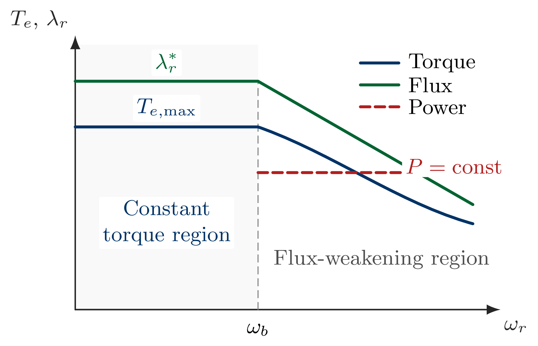 \caption{Torque-speed envelope showing the constant-torque and
field-weakening operating regions}
\caption{Torque-speed envelope showing the constant-torque and
field-weakening operating regions}
Voltage Limit Constraint
At rated speed and rated flux, the stator voltage can exceed
the maximum inverter output:
\[
V_s = \sqrt{V\qs^2 + V\ds^2} > V_{s,\max}
\]
- The dominant contribution is the back-EMF: \(\omegas(\Lm/\Lr)\lambdar\)
- To maintain \(V_s \le V_{s,\max}\), the flux must be reduced as \(\omegas\) increases
- Transition occurs at base speed \(\omega_b\) where \(V_s = V_{s,\max}\)
Practical Design Note
The relationship between phase and line voltage:\[
V_{LL} = \sqrt{3}\cdot\sqrt{2}\cdot V_s
\]
Dynamic Simulation Framework
Motivation and Model Components
{Purpose and Structure of Dynamic Simulation}Motivation
- Determine the transient response of the indirect vector-controlled drive to evaluate its suitability for a target application
- Avoid costly prototype build-and-test cycles
- Explore performance under different load profiles, reference trajectories, and parameter variations
- Validate controller design prior to hardware implementation
System Components Modelled
- Speed controller (PI with anti-windup)
- Vector controller (flux and torque computation)
- Inverter with switching logic (PWM / hysteresis)
- Induction machine (full nonlinear equations)
- Load (constant, fan, or pump torque profile)
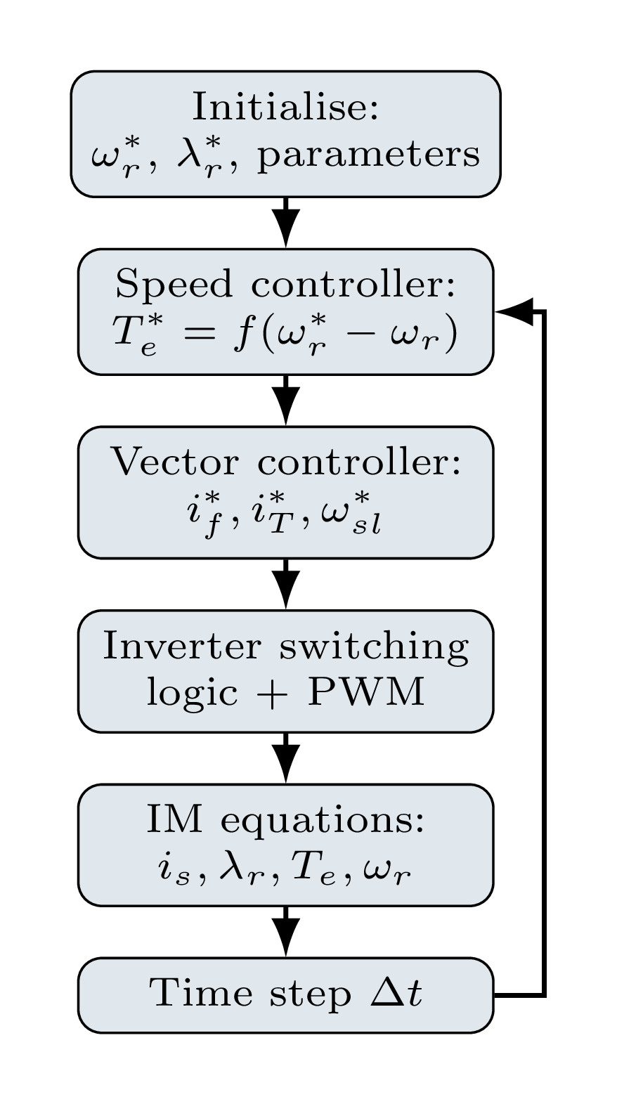 \caption{Flowchart for computation of the dynamic response of the
indirect vector-controlled induction motor drive}
\caption{Flowchart for computation of the dynamic response of the
indirect vector-controlled induction motor drive}
Full Nonlinear Machine Model
{Full Nonlinear Induction Machine Model}Complete Machine Equations in the Synchronous Reference Frame
Stator voltage equations:
\begin{align*}
v\qs &= \Rs\,\iqs + \frac{d}{dt}\!\left(\Ls\,\iqs + \Lm\,i_{qr}^e\right)
+ \omegas\!\left(\Ls\,\ids + \Lm\,i_{dr}^e\right)\\[3pt]
v\ds &= \Rs\,\ids + \frac{d}{dt}\!\left(\Ls\,\ids + \Lm\,i_{dr}^e\right)
- \omegas\!\left(\Ls\,\iqs + \Lm\,i_{qr}^e\right)
\end{align*}
\begin{align*}
0 &= \Rr\,i_{qr}^e + \frac{d}{dt}\!\left(\Lr\,i_{qr}^e + \Lm\,\iqs\right)
+ \omegasl\!\left(\Lr\,i_{dr}^e + \Lm\,\ids\right)\\[3pt]
0 &= \Rr\,i_{dr}^e + \frac{d}{dt}\!\left(\Lr\,i_{dr}^e + \Lm\,\ids\right)
- \omegasl\!\left(\Lr\,i_{qr}^e + \Lm\,\iqs\right)
\end{align*}
\[
J\,\frac{d\omegar}{dt} = \Te - T_L - B\omegar, \qquad
\Te = \frac{3P}{4}\,\Lm\!\left(\iqs\,i_{dr}^e - \ids\,i_{qr}^e\right)
\]
- All nonlinearities preserved — no linearisation applied
- Numerically integrated with 4th-order Runge–Kutta method
Simulation Results
CSI Drive Response
{Current-Source Indirect Vector Control — Transient Response}Step Speed Reversal — CSI Drive
Observable from simulation traces:
- Speed \(\omega_m\): smooth, fast tracking with no oscillatory response
- Rotor flux \(\lambda_m\): remains essentially constant during speed transients — decoupling maintained
- Torque \(T_e\): fast, high-magnitude response with well-defined limiter clipping during reversal
- Stator current \(i_{as\)}: magnitude varies cleanly; frequency changes smoothly with speed
Sinusoidal Speed Reference — CSI
The drive tracks a sinusoidal speed reference closely:- No phase lag in flux response
- Torque in phase with the speed derivative
- Stator current envelope follows the speed amplitude
VSI Drive Response
{Voltage-Source Indirect Vector Control — Transient Response}Step Speed Reversal — VSI Drive
Key observations:
- Faster speed command response compared to CSI (higher current bandwidth from inner \(dq\) current loops)
- Torque command \(T_e^*\) shows ideal limiter clipping
- Actual torque \(T_e\) tracks the command closely
- Flux \(\lambda_m\) remains constant throughout the reversal — flux and torque channels remain decoupled
- Stator current waveform shows natural PWM switching ripple
VSI vs.\ CSI — Performance Comparison
| lcc@{}} Feature | VSI | CSI |
| Current control | Inner PI | Direct |
| Torque bandwidth | Higher | Moderate |
| Flux regulation | Excellent | Excellent |
| Switching losses | Moderate | Lower |
| Industrial use | Dominant | Less common |
Performance Assessment
{Assessment of Vector-Controlled Drive Performance}Performance Metrics Achieved
- Decoupling: flux and torque independently controllable
- Torque bandwidth: \(>100\)\,Hz (set by current loop)
- Speed bandwidth: 10–50\,Hz (limited by inertia)
- Flux bandwidth: set by \(\Tr\) (deliberately slow)
- Zero-speed torque: full rated torque at standstill
- Four-quadrant operation: regenerative braking included
Conditions for Ideal Performance
All stated metrics assume:- Motor and controller parameters exactly matched
- Accurate rotor position measurement
- Sufficient inverter voltage headroom
- Operation within the linear magnetic range
Summary
{Summary — Lecture 4}- Steady-state analysis confirms that the indirect vector controller produces correct flux and torque when parameters are matched; the stator voltage at rated speed may necessitate flux weakening
- Two operating regions: constant-torque below \(\omega_b\) and constant-power (flux-weakening) above \(\omega_b\)
- Dynamic simulation uses the complete nonlinear induction machine model — stator, rotor, and mechanical equations — together with the full drive chain
- Simulation confirms: rotor flux remains constant during torque transients (decoupling verified), torque response is achieved in a few milliseconds, and speed tracking is smooth
- VSI drives show slightly higher bandwidth than CSI drives due to the inner \(dq\) current regulation loops
- Ideal performance degrades with parameter mismatch — quantified rigorously in Lecture~5