Lecture Series Overview
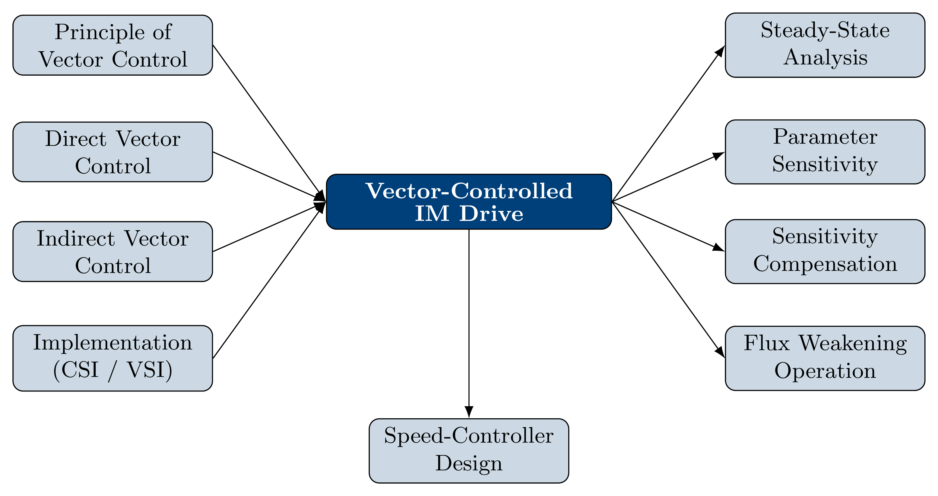
Eight Lecture Presentations
- Introduction & Principle of Vector Control
- Direct Vector Control
- Indirect Vector Control
- Steady-State Analysis & Drive Dynamics
- Parameter Sensitivity
- Parameter Compensation Strategies
- Flux-Weakening Operation
- Speed-Controller Design
Prerequisites
- Induction machine modelling (\(dq0\) theory)
- Power electronics and inverter topologies
- Classical control theory (PID, Bode, root locus)
- Fundamentals of electric drives
Reference Text
R Krishnan,
Electric Motor Drives: Modelling, Analysis and Control
, Prentice Hall, 2001.
Topic Map — Vector-Controlled Induction Motor Drives
Notation and Symbol Reference
Key Variables
| \(\iqs,\, \ids\) | \(q\)- and \(d\)-axis stator currents (sync frame) |
| \(\iT,\, \ifld\) | Torque- and field-producing stator current components |
| \(\lambda_r,\, \lambda_s\) | Rotor / stator flux linkage phasor magnitude |
| \(\thetaf\) | Field angle (rotor flux phasor position) |
| \(\omega_r,\, \omega_s\) | Rotor / synchronous electrical angular speed |
| \(\omega_{sl}\) | Slip speed \((\omega_s - \omega_r)\) |
| \(\Te\) | Electromagnetic torque |
Key Parameters
| \(\Rs,\, \Rr\) | Stator / rotor resistance per phase |
| \(\Ls,\, \Lr,\, \Lm\) | Stator, rotor, mutual inductance |
| \(\sigma = 1 - \Lm^2/(\Ls\Lr)\) | Total leakage coefficient |
| \(\Tr = \Lr/\Rr\) | Rotor time constant |
| \(\alpha = \Rr^*/\Rr\) | Rotor-resistance mismatch ratio |
| \(\beta = \Lm^*/\Lm\) | Mutual-inductance mismatch ratio |
| \(J,\, B\) | Rotor inertia / friction coefficient |
Superscripts and Subscripts
\[ \begin{aligned} e &\;-\; \text{synchronous frame} \\ s &\;-\; \text{stationary frame} \\ * &\;-\; \text{commanded (reference) value} \end{aligned} \]Motivation and Background
Limitations of Scalar Control
The Fundamental Problem
- Inverter-fed induction motor drives with scalar (\(V/f\)) control give good steady-state but poor dynamic performance.
- Root cause: the air-gap flux linkage phasor deviates from its set value in both magnitude and phase during transients.
- Flux deviations produce torque oscillations, which in turn produce speed oscillations.
- Large peak stator currents demand over-rated inverters.
High-Performance Applications Affected
- Robotic actuators and CNC machine tools
- Centrifuges and precision servos
- Metal-rolling mills
- Traction and process drives
The DC Machine Analogy
Separately-Excited DC Motor
- Field current \(i_f\) \(\to\) controls flux independently
- Armature current \(i_a\) \(\to\) controls torque independently
- Full decoupling is ensured by the commutator
- Only the magnitudes of \(i_f\) and \(i_a\) need to be controlled
\[ \Te = K_\phi\, i_f \cdot i_a \]
Induction Motor Challenge
- Stator current magnitude and phase must both be controlled
- No physical commutator — the inverter plays this role
- Coordinated control of magnitude, frequency, and phase is needed
- AC drives can achieve DC-like performance via vector control
Fundamental Insight
The stator current phasor can be resolved along the rotor flux axis : the component along \(\lambdar\) produces the field; the component perpendicular to \(\lambdar\) produces the torque. These two components can then be controlled independently.Benefits of Vector Control
Why Vector Control? — Performance and Practical Advantages
Performance Advantages
- Independent, instantaneous control of flux and torque
- Dynamic performance equivalent to — and in some respects superior to — separately-excited DC drives
- Minimal inverter peak-current over-rating
- Fast torque response comparable to DC servo drives
- Full rated torque achievable down to standstill
Practical Advantages of Using an IM
- Rugged, brushless, and low maintenance
- Lower cost and weight than equivalent DC machines
- Suitable for operation in harsh environments
- Extended speed range via flux weakening
- No risk of demagnetisation (unlike PM machines)
Principle of Vector Control
Reference Frame Transformation
Synchronous (\(dq\)) Reference Frame
The three-phase stator currents \(\{i_{as},\, i_{bs},\, i_{cs}\}\) are transformed to \(dq\) components in the
synchronous frame rotating at the field angle \(\thetaf\):
\[ \begin{bmatrix} \iqs \\ \ids \end{bmatrix} = \frac{2}{3} \begin{bmatrix} \sin\thetaf &
\sin\!\left(\thetaf - \tfrac{2\pi}{3}\right) & \sin\!\left(\thetaf + \tfrac{2\pi}{3}\right) \\[4pt]
\cos\thetaf & \cos\!\left(\thetaf - \tfrac{2\pi}{3}\right) & \cos\!\left(\thetaf +
\tfrac{2\pi}{3}\right) \end{bmatrix} \begin{bmatrix} i_{as} \\ i_{bs} \\ i_{cs} \end{bmatrix} \]
Stator current phasor magnitude
\[ i_s = \sqrt{\left(\iqs\right)^2 + \left(\ids\right)^2} \]
Stator phasor angle
\[ \theta_s = \tan^{-1}\!\left\{\frac{\iqs}{\ids}\right\} \]
- \(\iqs\) and \(\ids\) are DC quantities in steady state — no rotating phasors to track
- Low-bandwidth computational circuits suffice for their processing
Phasor Diagram and Field Alignment
Key Phasors and Angles
| \(\lambdar\) | Rotor flux linkage phasor |
| \(\thetaf\) | Field angle (rotor flux axis) |
| \(\theta_r\) | Rotor position angle |
| \(\theta_{sl}\) | Slip angle |
| \(\ifld = \ids\) | Field-producing component |
| \(\iT = \iqs\) | Torque-producing component |
\[ \thetaf = \theta_r + \theta_{sl} \]
\[ \theta_s = \thetaf + \theta_T \]
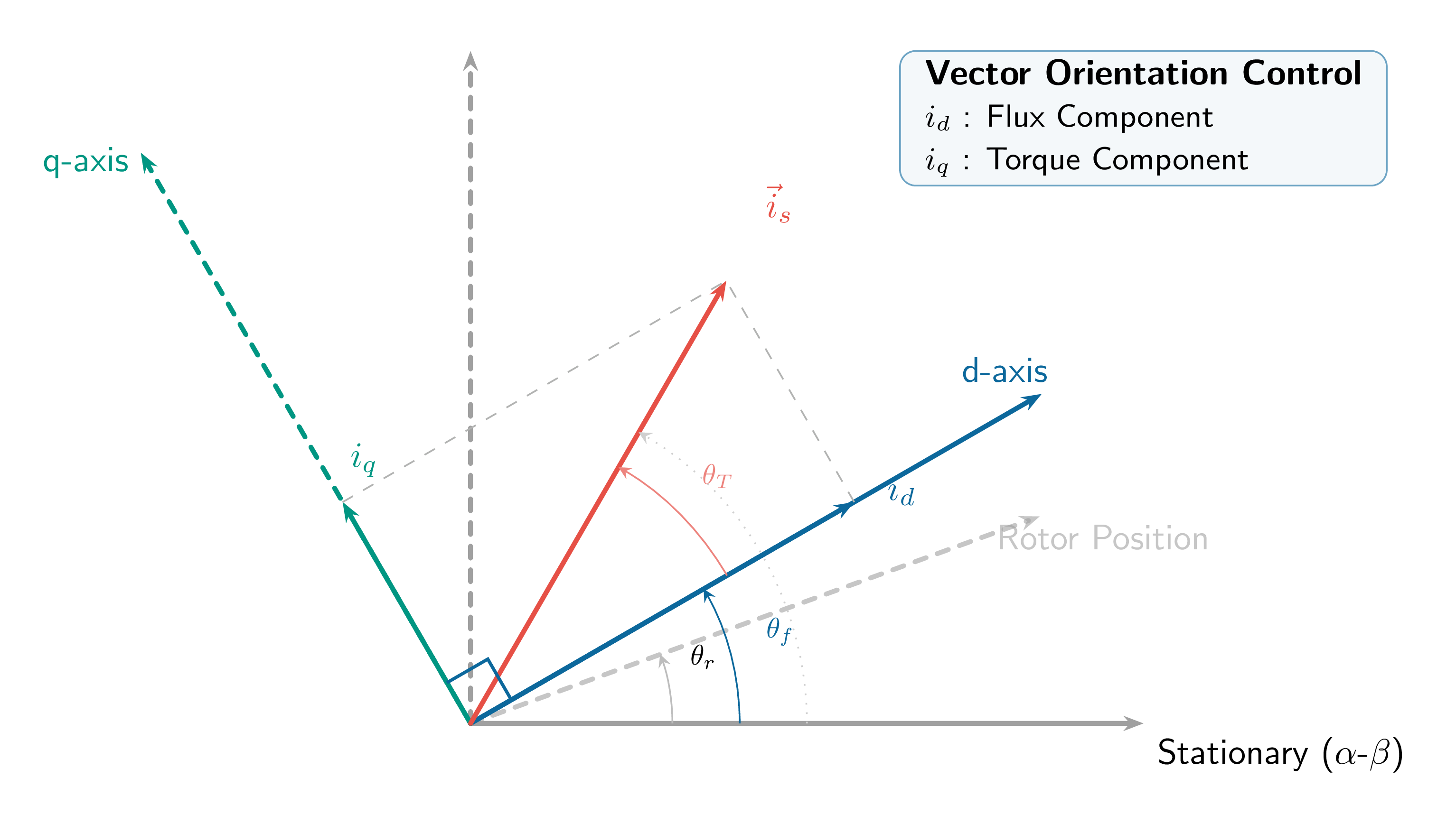
- \(\ifld \propto \lambdar\) (field-producing; DC in steady state)
- \(\Te \propto \lambdar \cdot \iT\) (torque-producing; DC in steady state)
Flux and Torque Decoupling
Fundamental Relationships
With the stator current phasor resolved
along
\(\lambdar\):
\begin{align*} \lambdar &\propto \ifld \\[4pt] \Te &\propto \lambdar \cdot \iT \propto \ifld
\cdot \iT \end{align*}
- \(\ifld\) and \(\iT\) are DC quantities in steady state
- They are independent control variables — exactly as in the separately-excited DC machine
- Independent bandwidth: torque channel is fast ; flux channel is slow (rotor time constant \(\Tr\))
Why DC Quantities Matter
- Signal-processing circuits need zero bandwidth in steady state
- No interaction between flux and torque channels
- Fast, independent torque control even at zero speed
- Eliminates the torque oscillation problem of scalar drives
Physical Interpretation
The inverter replaces the mechanical commutator: it controls both the magnitude and phase of the stator current phasor, decoupling the flux and torque channels by precisely injecting \(\ifld\) and \(\iT\) at the optimum \(90°\) spatial orientation.The Field Angle
Definition of Field Angle \(\thetaf\)
The position of the rotor flux linkage phasor measured from the stationary reference axis:
\[ \thetaf = \theta_r + \theta_{sl} \qquad \text{equivalently} \qquad \thetaf = \int \!\left(\omegar +
\omegasl\right)\mathrm{d}t = \int \omegas\,\mathrm{d}t \]
Direct Vector Control
- \(\thetaf\) obtained by directly measuring terminal voltages and currents, or by using flux-sensing windings or Hall-effect sensors
- No rotor position sensor strictly required
- Sensitive to stator resistance variation at low speed
Indirect Vector Control
- \(\thetaf\) computed using rotor position measurement and partial estimation from machine parameters
- Slip angle \(\theta_{sl}\) estimated from rotor equations
- No direct flux sensor needed
- Sensitive to rotor parameter variation
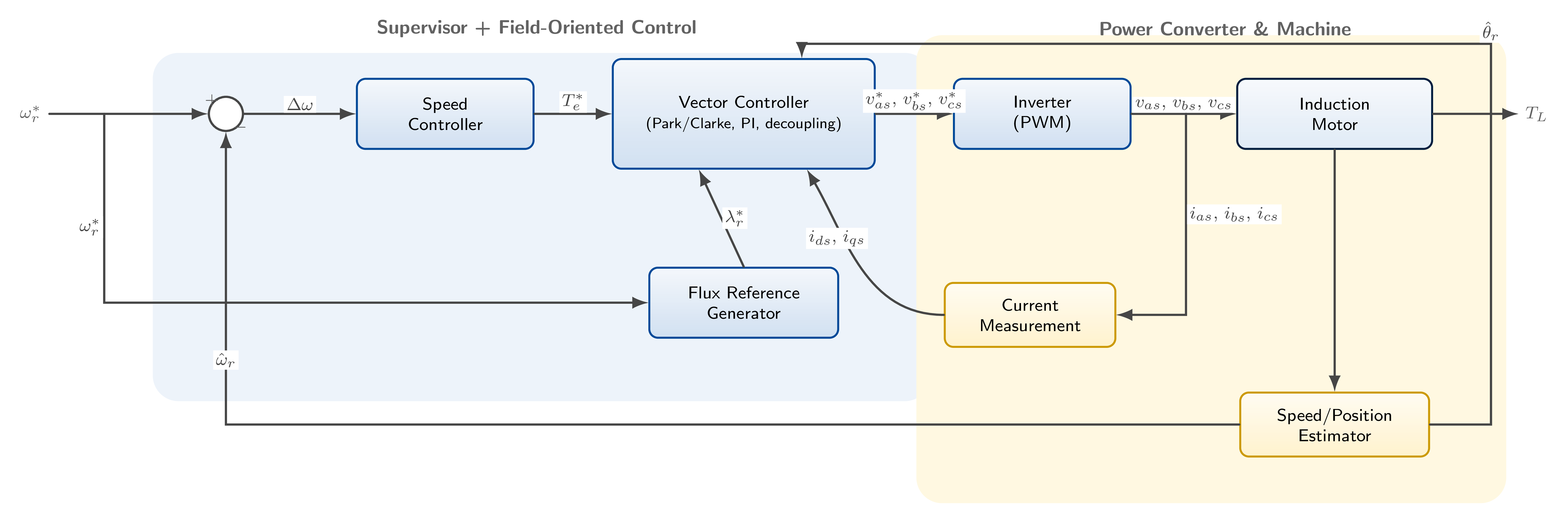
Vector Control Algorithm
- Obtain field angle \(\thetaf\) (direct measurement or indirect computation)
- Compute field-producing current command from the required rotor flux: \(\ifld^* = f(\lambdar^*,\, \Lm)\)
- Compute torque-producing current command from the torque command: \(\iT^* = T_e^*/\!\left(K_{te}\lambdar^*\right)\)
- Compute stator current phasor magnitude: \(i_s^* = \sqrt{(\ifld^*)^2 + (\iT^*)^2}\)
- Compute torque angle: \(\theta_T = \tan^{-1}\!\left(\iT^*/\ifld^*\right)\)
- Obtain stator phasor angle: \(\theta_s = \thetaf + \theta_T\)
- Apply inverse transform (\(dq \to abc\)) to generate three-phase current commands
- Synthesise via inverter \(\Rightarrow\) commanded \(\lambdar\) and \(\Te\) produced
Critical Requirement
The accuracy of all computed quantities depends entirely on the accuracy of the field angle \(\thetaf\). Any error in \(\thetaf\) leads to imperfect decoupling of the flux and torque channels.Notation
- \(K_{te} = \tfrac{3P\Lm}{4\Lr}\) torque constant
- \(P\) number of poles
Block Diagram and Classification
Classification of Vector Control Schemes
| Criterion | Direct | Indirect |
| Field angle source | Flux sensors / voltage model | Rotor position + slip estimation |
| Flux measurement | Required | Not required |
| Primary sensitivity | Stator resistance \(\Rs\) | Rotor time constant \(\Tr\) |
| Industrial prevalence | Less common | Dominant |
Summary
Key Takeaways
- Scalar control gives poor dynamic response due to uncontrolled flux phasor deviations during transients
- Vector (field-oriented) control resolves the stator current phasor along the rotor flux axis, achieving DC-machine equivalent performance
- The field angle \(\thetaf\) is the cornerstone of vector control
- \(\ifld\) and \(\iT\) become independent DC control variables — flux and torque channels are fully decoupled
- Two implementation strategies exist: direct and indirect vector control
Coming Up
- Lecture 8B : Direct Vector Control — flux sensing methods, CSI and VSI implementations, space vector modulation
- Lecture 8C : Indirect Vector Control — rigorous derivation, complete scheme, implementation details
- Lectures 8D–H : Steady-state analysis, parameter sensitivity, compensation strategies, flux weakening, and speed-controller design
Fundamental Equation
\[ \Te = K_{te}\,\lambdar\,\iT = K_{te}\,\Lm\,\ifld\,\iT \]