Overview of Direct Vector Control

Direct Vector Control — Defining Characteristic

What Makes It ``Direct''

In direct vector control, the field angle \(\thetaf\) is obtained by measuring or directly computing the flux linkages from terminal electrical quantities or dedicated sensors. No knowledge of the rotor position is strictly required.

Block Structure with Current-Source Inverter

Speed error through PI controller \(\to\) torque command \(T_e^*\)
Flux reference \(\lambdar^*\): held at rated value up to base speed; reduced inversely with speed above base (field weakening)
Vector controller generates \(\ifld^*\), \(\iT^*\), and \(\theta_s^*\)
CSI enforces the current commands directly

Field-Weakening Strategy

\[ \lambdar^* = \begin{cases} \lambda_b & 0 \le \omegar \le \omega_b \\[4pt] \dfrac{\omega_b}{|\omegar|}\lambda_b & |\omegar| > \omega_b \end{cases} \]

Keeps induced EMF within the inverter voltage limit
Extends the speed range at reduced flux

Block Diagram — Direct Vector Controller with CS

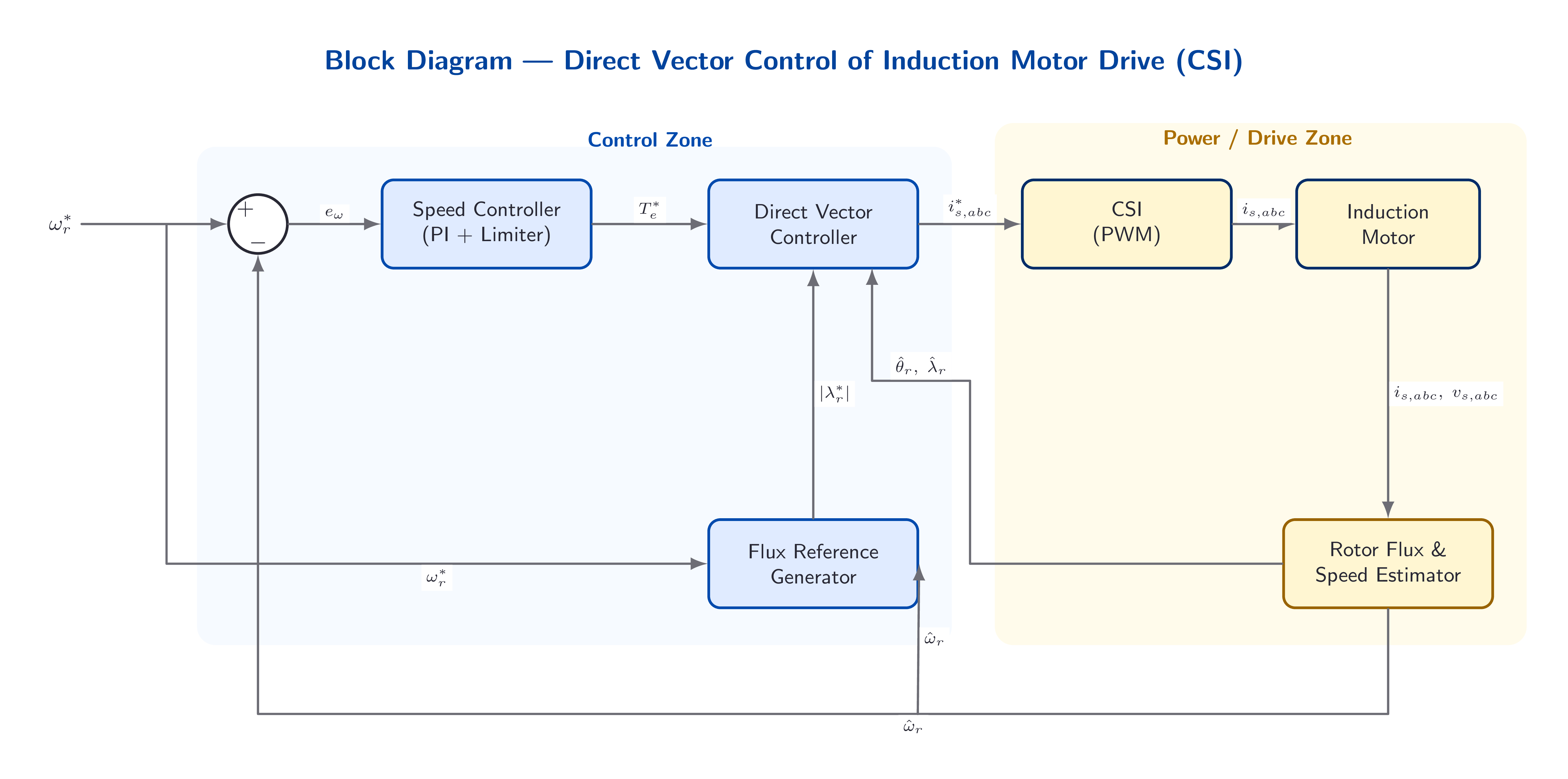
Lecture Figure — Block diagram of direct vector controller with current-source inverter showing feedback paths for flux magnitude and field angle

The flux estimator returns both \(|\lambdar|\) and the field angle \(\thetaf\)
All inner-loop feedback paths operate at high bandwidth

Flux Estimation Methods

Voltage Model

Flux Estimation — Voltage Model (Terminal Quantities)

Stator Voltage Equations in the Stationary Frame

\[ v_{qs}^s = \Rs\,i_{qs}^s + \frac{d\lambda_{qs}^s}{dt}, \qquad v_{ds}^s = \Rs\,i_{ds}^s + \frac{d\lambda_{ds}^s}{dt} \]

Integrating to obtain the stator flux linkages:

\[ \lambda_{qs}^s = \int\!\left(v_{qs}^s - \Rs\,i_{qs}^s\right)\mathrm{d}t, \qquad \lambda_{ds}^s = \int\!\left(v_{ds}^s - \Rs\,i_{ds}^s\right)\mathrm{d}t \]

Rotor flux linkages obtained from stator flux and currents:

\[ \lambda_{qr}^s = \frac{\Lr}{\Lm}\!\left(\lambda_{qs}^s - \sigma\Ls\,i_{qs}^s\right), \qquad \lambda_{dr}^s = \frac{\Lr}{\Lm}\!\left(\lambda_{ds}^s - \sigma\Ls\,i_{ds}^s\right) \]

Field Angle Computation

\[ \thetaf = \tan^{-1}\!\!\left(\frac{\lambda_{qr}^s}{\lambda_{dr}^s}\right), \qquad |\lambdar| = \sqrt{(\lambda_{qr}^s)^2 + (\lambda_{dr}^s)^2} \]

Limitation at Low Speed

At low speed, \(v_s \approx \Rs i_s\), so errors in \(\Rs\) dominate the flux estimate. Temperature rise of 100\,°C can double the winding resistance.

Sensing Coils and Hall Sensors

Flux Estimation — Sensing Coils and Hall-Effect Sensors

Flux-Sensing (Search) Coils

Two sets of search coils placed in stator slots, \(90°\) electrically displaced
Induced EMF proportional to the rate of change of stator flux:
\[ \lambda_{qs} = \int e_{qs}\,\mathrm{d}t, \quad \lambda_{ds} = \int e_{ds}\,\mathrm{d}t \]
No \(\Rs\) dependence — accurate at all speeds
Galvanically isolated from the power circuit
Requires integration; sensitive to offset and drift

Hall-Effect Sensors

Placed in the air gap to measure flux density \(B\) directly
Provide instantaneous flux — no integration required
Give both magnitude and angle of the flux phasor
Mechanically fragile and limited in thermal range
Suitable for well-designed motor housings

Comparison of Flux Estimation Methods

Method	Speed range	\(\Rs\) dependent	Remarks
Voltage model	Low speed problematic	Yes	Simple; needs compensation
Search coils	All speeds	No	Requires integrator circuit
Hall sensors	All speeds	No	Fragile; air-gap access needed

Direct Vector Control with Voltage-Source Inverter

Current Regulation

Implementation with Voltage-Source Inverter

Current Regulation via VSI

Current commands \(i_{qs}^{e*}\) and \(i_{ds}^{e*}\) generated by the vector controller
\(dq\) current errors produce voltage commands \(v_{qs}^{e*}\) and \(v_{ds}^{e*}\)
Inverse transform (\(e \to s\) frame) converts to three-phase voltage commands
VSI synthesises the commanded voltages via PWM

Cross-Coupling in the Synchronous Frame

The stator voltage equations contain coupling terms:

\begin{align*} v_{qs}^e &= (R_s + \sigma L_s p)\,\iqs + \omegas\sigma L_s\,\ids + \omegas\frac{\Lm}{\Lr}\lambdar \\[3pt] v_{ds}^e &= (R_s + \sigma L_s p)\,\ids - \omegas\sigma L_s\,\iqs \end{align*}

Feed-Forward Decoupling

Cross-coupling terms are cancelled by feed-forward:

Feed-forward voltage \(\omegas\sigma\Ls\ids\) added to \(q\)-axis reference
Feed-forward voltage \(\omegas\sigma\Ls\iqs\) subtracted from \(d\)-axis reference
Back-EMF term \(\omegas(\Lm/\Lr)\lambdar\) also cancelled

Result: independent \(dq\) current control with first-order \(R_s\)-\(\sigma L_s\) plant dynamics.

Space Vector Modulation

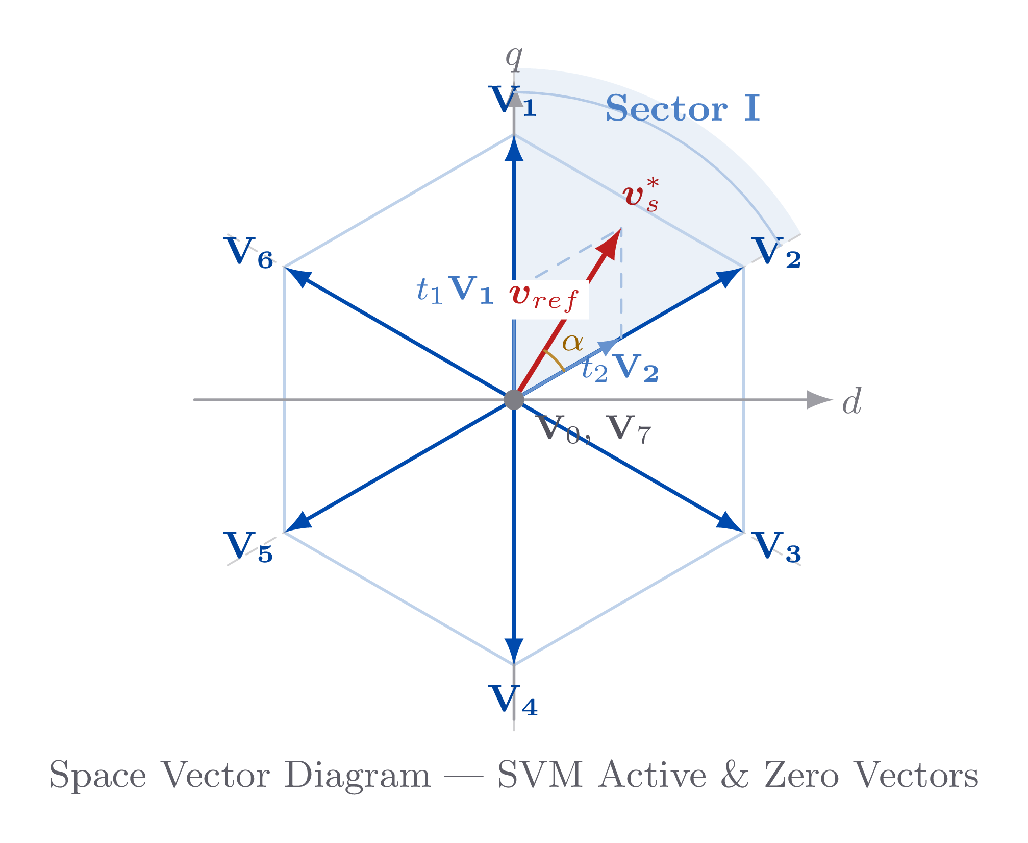
Principle of SVM

A three-phase VSI produces six active and two zero voltage vectors forming a regular hexagon
The desired voltage vector \(v_s^*\) is synthesised from the two adjacent active vectors weighted by duty cycles
The remaining switching period uses zero vectors
Duty cycles determined by projection of \(v_s^*\) onto the two nearest vectors

Advantages over Carrier-Based PWM

Higher fundamental voltage capability\newline (up to \(V_{dc}/\sqrt{3}\) vs.\ \(V_{dc}/2\))
Minimised switching losses for given switching frequency
Lower voltage and current ripple
Direct digital implementation; no explicit carrier needed

SVM — Flux Trajectory Control

Stator-Flux-Based Switching Selection

The desired stator flux \(\lambdas^*\) has magnitude \(\lambda_s\) and position \(\theta_{fs}\) within one of six sextants
The influencing voltage vector is identified from the current sextant position
Two adjacent vectors applied as time fractions within the switching period to track the reference trajectory
Zero vectors inserted to complete the period

Torque Control via Flux Trajectory

Air-gap torque: \(\Te \propto |\lambdas|\cdot|\lambdar|\sin\delta\) where \(\delta\) is the load angle
Controlling \(|\lambdas|\) and its rotational rate (via voltage vector selection) directly controls torque
This principle forms the basis of Direct Torque Control (DTC)

Stator-Resistance Sensitivity and Compensation

Effect of Stator Resistance Variation

Stator-Resistance Sensitivity

Effect of \(\Rs\) Variation on Flux Estimation

The voltage-model estimator uses:
\[ \hat{\lambda} = \int\!\left(v_s - \hat{R}_s\,i_s\right)\mathrm{d}t \]
At low speed: \(v_s \approx \hat{R}_s i_s\), so an error in \(\hat{R}_s\) dominates the flux estimate
Temperature rise of 100°C can double the winding resistance
\(\Rs\) mismatch causes:
1. Flux magnitude error
2. Torque magnitude error
3. Field angle \(\thetaf\) drift
Instability is possible at very low speeds

Instability Mechanism

Under rapidly decreasing \(\Rs\) (e.g.\ motor cooling):

Estimated \(\hat{R}_s > R_s\) actual
Flux estimate diverges from true value
Torque oscillates uncontrollably
Stator current may saturate the inverter

The drive can become unstable within a few seconds — unacceptable in servo applications.

Adaptive Compensation

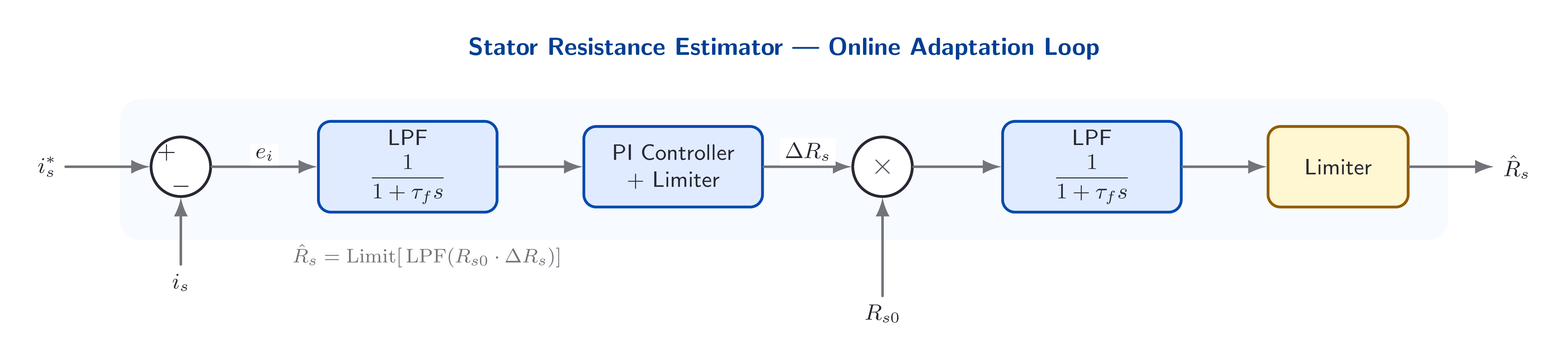
Adaptive Stator-Resistance Compensator

Operating Principle

The error between the commanded current \(i_s^*\) and the actual current \(i_s\) is filtered and processed through a PI controller
The PI output \(\Delta R_s\) updates the estimated resistance:
\[ \hat{R}_s = R_{s0} + \Delta R_s \]
A low-pass filter removes high-frequency PWM noise
A second filter and limiter prevent windup and oscillatory behaviour in the adaptation loop

Adaptive Compensator

Result

The adaptive compensator tracks \(\Rs\) changes continuously, maintaining stable torque control throughout the flux-weakening speed range.

Summary

Key Points

The field angle is obtained directly from flux measurement: voltage model, search coils, or Hall sensors
Compatible with both CSI and VSI inverters
VSI implementation requires feed-forward decoupling of cross-coupling terms
SVM offers superior modulation quality compared to carrier-based PWM
The principal weakness is \(\Rs\) sensitivity of the voltage model at low speed
Adaptive compensation restores performance across the full operating temperature range

Next Lecture — Indirect Vector Control

No flux sensors required
Field angle computed from rotor position and estimated slip angle
More widely used in industrial drives
Sensitivity shifts from \(\Rs\) to rotor parameters

Key Distinction

Direct VC is preferred when low-speed performance is essential and hardware sensor integration is feasible. It eliminates parameter uncertainty in the torque loop at the cost of flux sensor hardware.