The Compensation Problem
{Compensation Philosophy and Challenges}Goal
Minimise the degradation of vector control performance caused
by motor–controller parameter mismatch by adapting the
controller parameters to track the actual motor parameters
in real time, without interrupting drive operation.
Fundamental Challenges
- Direct parameter measurement during operation is generally impractical (no rotor access in a squirrel-cage motor)
- Most adaptation algorithms are themselves sensitive to other machine parameters
- Adaptation bandwidth is limited by the signal bandwidth available in the drive signals
- Performance near zero speed is a universal limitation of all estimation-based methods
Two Adaptation Strategies
Direct strategy:
- Monitor alignment of the flux and torque-producing axes
- Use the orientation error directly to update \(\Rr^*\)
- Measure a terminal quantity sensitive to \(\Rr\) (e.g., modified reactive power)
- Infer parameter variation from observable electrical signals
- No flux sensor or observer required
Direct Axis-Alignment Method
{Principle of Axis-Alignment Detection}Condition for Perfect Field Orientation
Perfect vector control requires:
\[
\lambda_{qr}^e = 0
\quad\Longleftrightarrow\quad
\text{\(q\)-axis rotor flux equals zero}
\]
Detection and Adaptation Scheme
- Compute \(\lambda_{qr}^e\) from measured stator currents and the estimated flux
- A nonzero \(\lambda_{qr}^e\) is the alignment error
- Use this error to adapt \(\Rr^*\):
\[ \frac{d\Rr^*}{dt} = -K_{\mathrm{adapt}}\cdot\lambda_{qr}^e\cdot\iqs \]
- The update law drives \(\lambda_{qr}^e \to 0\) in steady state
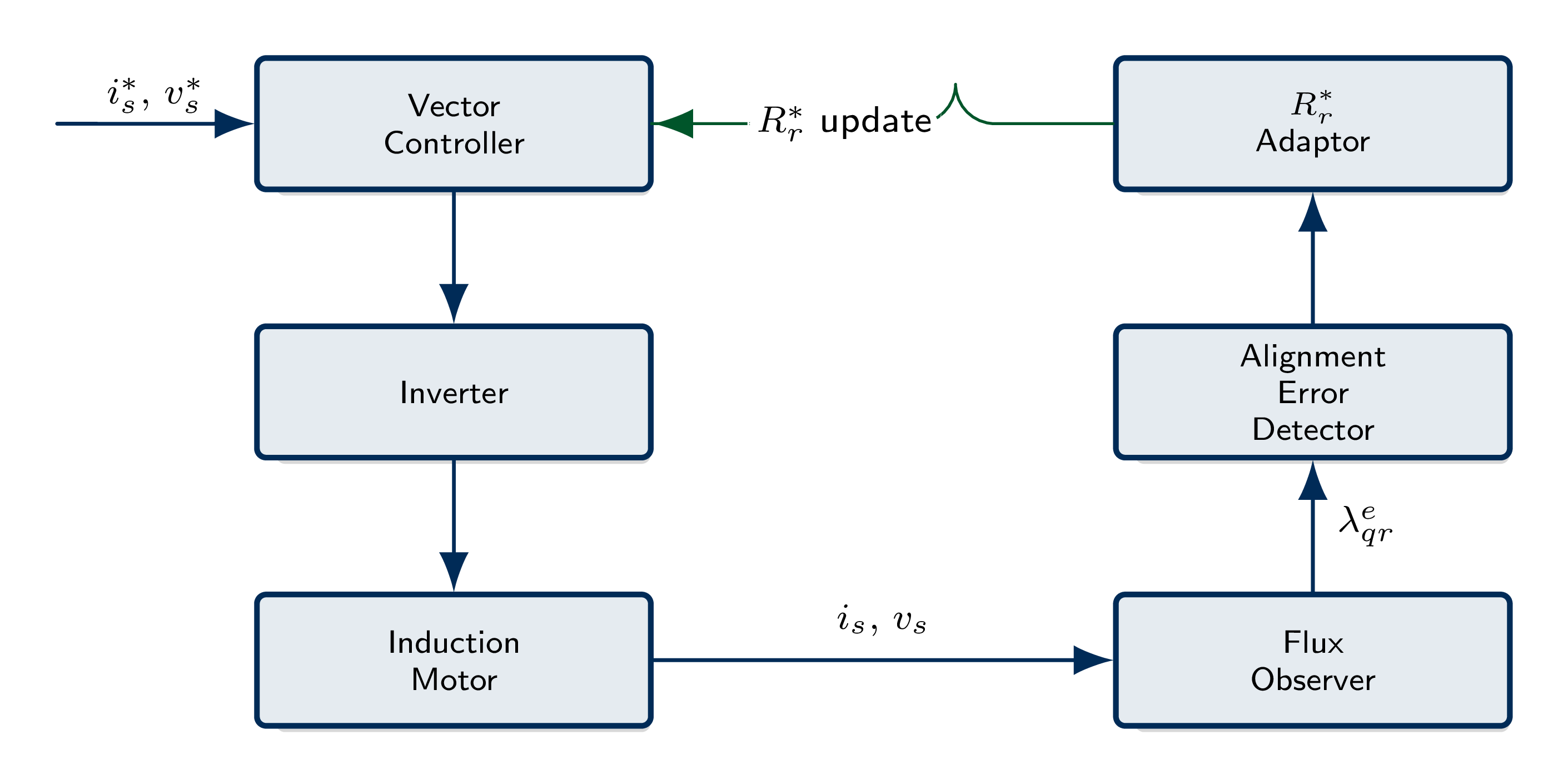 \caption{Block diagram of the axis-alignment detection and
\(\Rr^*\) adaptation scheme}
\caption{Block diagram of the axis-alignment detection and
\(\Rr^*\) adaptation scheme}
- No additional hardware beyond current sensors
- Convergence rate set by \(K_{\mathrm{adapt}}\)
Reactive Power Based Method
{Modified Reactive Power — Concept and Adaptation Law}Why Reactive Power?
The modified reactive power \(Q_m\) of the induction motor,
defined as the cross-product of stator voltage and current
in the stationary frame:
\[
Q_m = v_{ds}^s\,i_{qs}^s - v_{qs}^s\,i_{ds}^s
\]
- \(Q_m\) is sensitive to both \(\Lm\) and \(\Rr\)
- The sign of \((Q_m^* - Q_m)\) changes when \(\Rr^*\) crosses the true value of \(\Rr\)
- Reference \(Q_m^*\) from the controller model is compared to the measured \(Q_m\)
- The error \(\Delta Q_m = Q_m^* - Q_m\) drives adaptation
PI Adaptation Law
\[
\Delta Q_m \propto \left(\Rr^* - \Rr\right)
\]
\[
\Rr^*(s) = \left(K_p + \frac{K_i}{s}\right)\Delta Q_m(s)
\]
Key Advantage
Computed entirely from terminal measurements — no rotor flux observer or shaft position sensor required.Rotor Flux Deviation Method
{Rotor Flux Deviation as the Error Signal}Flux Deviation Principle
If the field angle \(\thetaf\) is in error due to \(\Rr\) mismatch:
- \(\lambda_{qr}^e \ne 0\) — nonzero quadrature rotor flux
- The ratio of \(q\)- to \(d\)-axis flux equals \(\tan(\Delta\theta)\) where \(\Delta\theta\) is the field angle error
- In steady state, this ratio is proportional to \((\alpha - 1)\):
\[
\frac{\lambda_{qr}^e}{\lambda_{dr}^e}
\approx \frac{(\alpha - 1)\,\omegasl^*\Tr}{1 + \alpha(\omegasl^*\Tr)^2}
\]
Implementation
- Estimate \(\lambda_{qr}^e\) from measured stator currents and rotor position
- Pass through a low-pass filter to remove PWM noise
- A PI controller drives \(\lambda_{qr}^e \to 0\) by adjusting \(\omegasl^*\) (equivalently \(\Rr^*\))
- Converges in a few rotor time constants
Practical Note
Flux observers require accurate \(\Ls\) and \(\Lm\) — residual errors from these induce a small bias offset but do not cause instability of the adaptation loop.MRAS Rotor-Resistance Identification
MRAS Framework
{MRAS Concept and Framework}MRAS Structure
- Reference model: uses measured quantities (stator currents, voltages) — has no \(\Rr\) dependence
- Adaptive model: uses the controller \(\Rr^*\) — its output depends on \(\Rr^*\)
- Error signal: difference between the two model outputs
- Adaptation mechanism: adjusts \(\Rr^*\) to drive the error to zero
Choice of Comparison Variable
Rotor flux linkages are used:
\[
\varepsilon = \hat{\lambda}_{qr}^{s\,(\mathrm{ref})}
- \hat{\lambda}_{qr}^{s\,(\mathrm{adapt})}
\]
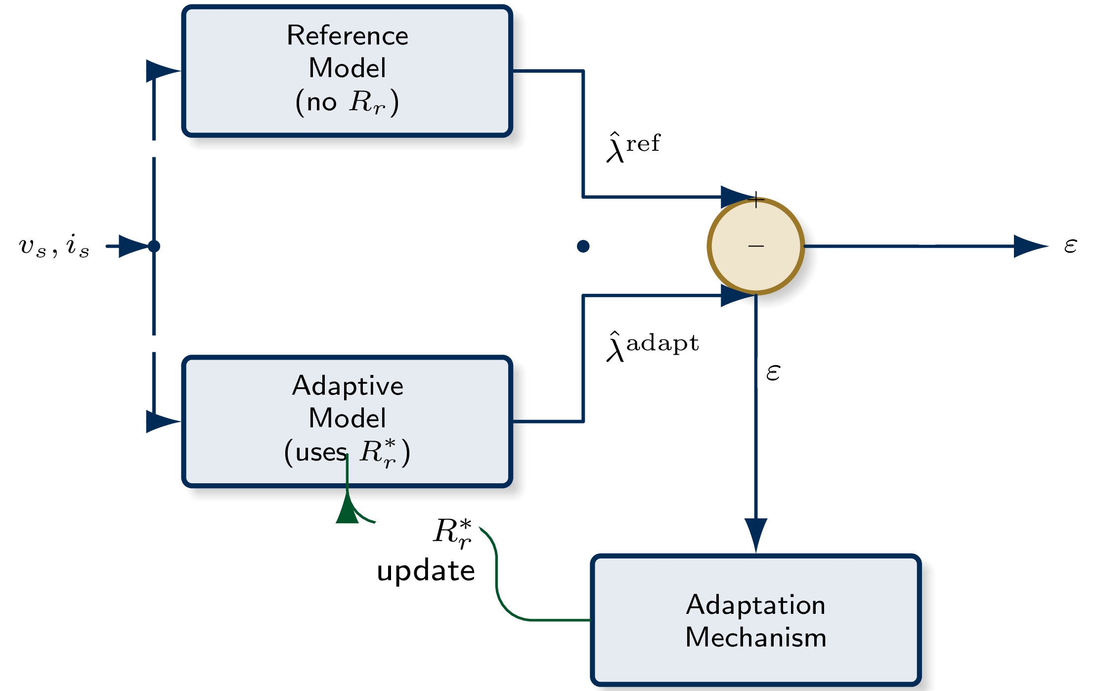 \caption{Block diagram of the MRAS framework for online
rotor-resistance identification}
\caption{Block diagram of the MRAS framework for online
rotor-resistance identification}
Popov Stability and Adaptation Law
{MRAS Adaptation Laws — Popov Hyperstability}Popov's Hyperstability Criterion
The MRAS is asymptotically stable if and only if the
adaptation law satisfies Popov's inequality:
\[
\int_0^t \varepsilon^{\mathsf{T}}\cdot w\,\mathrm{d}\tau \ge -\gamma^2,
\quad \forall\, t \ge 0
\]
Resulting Adaptation Law for \(\Rr^*\)
\[
\frac{d\Rr^*}{dt} = -K_1\,\varepsilon\cdot\phi_r
- K_2\int\!\varepsilon\cdot\phi_r\,\mathrm{d}t
\]
- \(\phi_r\): state component of the adaptive model proportional to \(\Rr^*\)
- \(K_1, K_2 > 0\): design gains (proportional and integral)
- Convergence guaranteed by Popov's criterion
Properties of MRAS Adaptation
- Global asymptotic stability proven via Lyapunov and Popov methods
- Converges to the correct \(\Rr\) regardless of initial error
- Adaptation rate tunable independently via \(K_1\), \(K_2\)
- Works for both increasing and decreasing \(\Rr\)
- Not excitation-dependent at non-zero speed
Fundamental Limitation
The MRAS fails at zero speed where the reference model becomes unobservable — a fundamental limitation shared by all estimation-based methods.Comparison and Summary
{Comparative Assessment of Compensation Methods}| lccccc@{}} Method | Sensors | Additional param. | Zero speed | Complexity | Stability |
| Axis alignment | \(i_s\), \(v_s\) | \(\Ls\), \(\Lm\) | No | Moderate | Conditional |
| Reactive power | \(i_s\), \(v_s\) | \(\Ls\), \(\Lm\) | No | Low | Conditional |
| Flux deviation | \(i_s\), \(\theta_r\) | \(\Ls\) | No | Moderate | Conditional |
| MRAS | \(i_s\), \(v_s\) | \(\Ls\), \(\Lm\) | No | High | Global (Popov) |
Common Limitations
- All methods fail near zero speed (universal observability constraint)
- All depend on some additional known parameters
- Slow adaptation bandwidth (governed by \(\Tr\))
- Cannot simultaneously handle \(\Rr\) and \(\Lm\) changes
Practical Guidance
- Parameter compensation is essential for robust vector control in thermally demanding environments
- MRAS offers the strongest theoretical stability guarantee
- The reactive power method is simplest to implement
- Hybrid strategies combining multiple signals improve reliability across the full operating range