Derivation of the Indirect Vector-Control Scheme
Rotor Equations and Orientation Condition
{Starting Point — Rotor Voltage Equations}Rotor Equations in the Synchronous Reference Frame
Assuming a current-source inverter (stator dynamics neglected):
\begin{align*}
R_r i_{qr}^e + \frac{d\lambda_{qr}^e}{dt} + \omegasl\lambda_{dr}^e &= 0 \\[4pt]
R_r i_{dr}^e + \frac{d\lambda_{dr}^e}{dt} - \omegasl\lambda_{qr}^e &= 0
\end{align*}
\begin{align*}
\lambda_{qr}^e &= \Lm\,\iqs + \Lr\,i_{qr}^e \\[4pt]
\lambda_{dr}^e &= \Lm\,\ids + \Lr\,i_{dr}^e
\end{align*}
Field-Orientation Condition
Align the \(d\)-axis of the synchronous frame with the rotor flux phasor:\[
\lambdar = \lambda_{dr}^e, \qquad \lambda_{qr}^e = 0, \qquad
\frac{d\lambda_{qr}^e}{dt} = 0
\]
Decoupled Equations after Orientation
{Decoupled Rotor Equations after Field Orientation} Substituting the orientation conditions into the rotor equations:Slip-Speed Equation — from \(q\)-axis
\[
\omegasl = \frac{\Rr\,\iqs}{\lambdar} = \frac{1}{\Tr}\cdot\frac{\iqs}{\ids}
\]
Rotor Flux Dynamics — from \(d\)-axis
Using \(i_{dr}^e = (\lambdar - \Lm\ids)/\Lr\):
\[
\Tr\,\frac{d\lambdar}{dt} + \lambdar = \Lm\,\ids
\]
- Rotor flux \(\lambdar\) is a first-order lag response to the field-producing current \(\ids = \ifld\)
- Time constant \(= \Tr\) (typically 0.1–1\,s)
- This is the slow control channel
Significance
The two equations are completely decoupled when \(\lambda_{qr}^e = 0\) — torque can be changed instantaneously without disturbing the rotor flux.Torque Equation and Transfer Functions
{Electromagnetic Torque and Control Transfer Functions}Electromagnetic Torque Expression
\[
\Te = \frac{3P}{4}\cdot\frac{\Lm}{\Lr}\,\lambdar\,\iqs
= K_{te}\,\lambdar\,\iT
\]
- \(\lambdar\) — controlled via \(\ids\) (slow)
- \(\iT = \iqs\) — torque-producing current (fast)
Transfer Functions of the Two Channels
Flux channel (slow):
\[
\frac{\lambdar(s)}{\ifld(s)} = \frac{\Lm}{1 + s\Tr}
\]
\[
\frac{\Te(s)}{\iT(s)} = K_{te}\,\lambdar \approx \text{const}
\]
- Torque responds instantaneously to \(\iT\)
- Flux responds with time constant \(\Tr\)
- No coupling between channels when \(\lambda_{qr}^e = 0\)
Coordinate Transformation and Field Angle
{Coordinate Transformation for Indirect Control}Three-Phase to \(dq\) Transformation at Field Angle \(\thetaf\)
\[
\begin{bmatrix} \iqs \\ \ids \end{bmatrix}
= \frac{2}{3}
\begin{bmatrix}
\cos\thetaf & \cos\!\left(\thetaf-\tfrac{2\pi}{3}\right) &
\cos\!\left(\thetaf+\tfrac{2\pi}{3}\right)\\[4pt]
\sin\thetaf & \sin\!\left(\thetaf-\tfrac{2\pi}{3}\right) &
\sin\!\left(\thetaf+\tfrac{2\pi}{3}\right)
\end{bmatrix}
\begin{bmatrix}i_{as}\\i_{bs}\\i_{cs}\end{bmatrix}
\]
Field Angle Computation (Indirect)
\[
\thetaf = \theta_r + \theta_{sl}, \qquad
\theta_{sl} = \int\!\omegasl\,\mathrm{d}t
= \int\!\frac{\iqs}{\Tr\,\ids}\,\mathrm{d}t
\]
- \(\theta_r\) measured by shaft encoder or resolver
- \(\theta_{sl}\) computed from motor parameters and commanded currents
No Flux Sensor Required
- Field angle is estimated, not measured
- Only rotor position \(\theta_r\) is needed
- Accuracy depends on \(\Tr = \Lr/\Rr\)
- Parameter mismatch causes imperfect decoupling (analysed in detail in Lecture~5)
The Indirect Vector-Control Scheme
Current Commands
{Current Commands from the Vector Controller}Commanded Quantities (Derived from Rotor Equations)
Field-producing current command:
\[
\ifld^* = \frac{(1 + s\Tr^*)}{\Lm^*}\,\lambdar^*
\]
\[
\iT^* = \frac{T_e^*}{K_{te}^*\,\lambdar^*}
\]
\[
\omegasl^* = \frac{1}{\Tr^*}\cdot\frac{\iT^*}{\ifld^*}
= \frac{\Lm^*\,\iT^*}{\Tr^*\,\lambdar^*}
\]
Three-Phase Current Synthesis
Stator current phasor magnitude:
\[
i_s^* = \sqrt{(\ifld^*)^2+(\iT^*)^2}
\]
\[
\begin{bmatrix}i_{as}^*\\i_{bs}^*\\i_{cs}^*\end{bmatrix}
= i_s^*\begin{bmatrix}
\sin\theta_s^*\\\sin(\theta_s^*-\tfrac{2\pi}{3})\\\sin(\theta_s^*+\tfrac{2\pi}{3})
\end{bmatrix}
\]
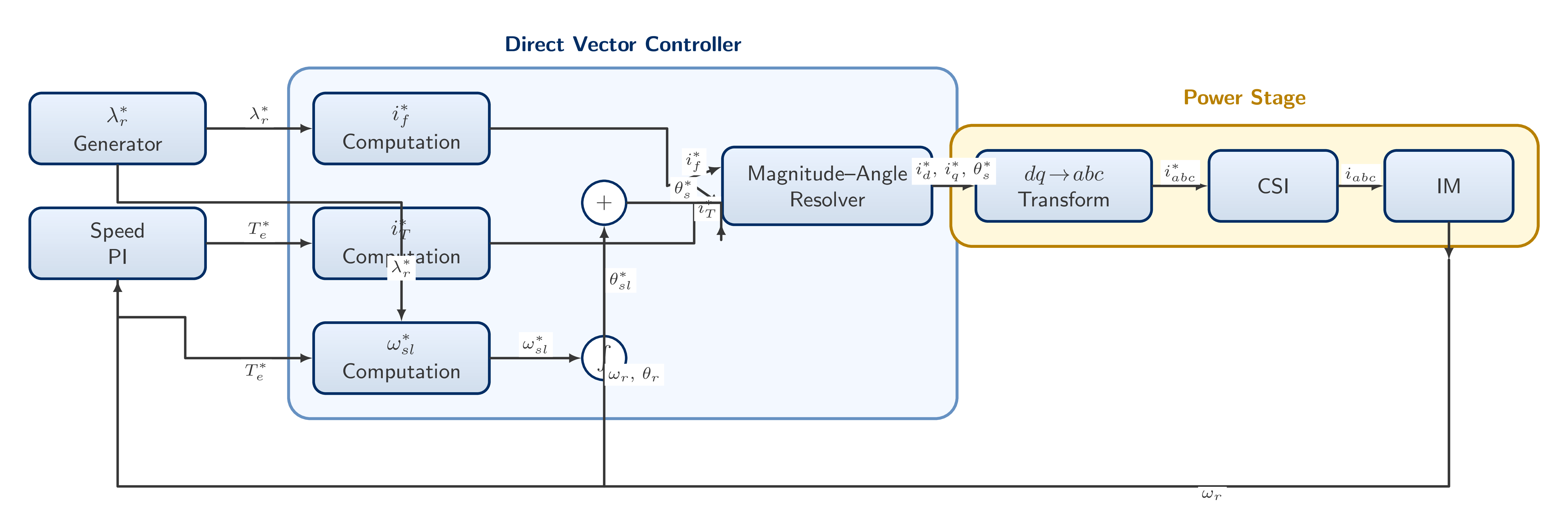 \caption{Complete block diagram of the indirect vector controller showing
the slip-speed computation, field-angle accumulation, and
three-phase current synthesis}
\caption{Complete block diagram of the indirect vector controller showing
the slip-speed computation, field-angle accumulation, and
three-phase current synthesis}
Implementation Details
Flux Command and Field Weakening
{Complete Implementation — Flux Command and Speed Controller}Flux Reference Schedule
\[
\lambdar^* =
\begin{cases}
\lambda_b & |\omegar| \le \omega_b \\[4pt]
\dfrac{\omega_b}{|\omegar|}\lambda_b & |\omegar| > \omega_b
\end{cases}
\]
- Below base speed: constant-flux (constant-torque) region
- Above base speed: flux reduced \(\propto 1/\omegar\) (constant-power region)
- Extends the speed range without exceeding inverter voltage or current ratings
Torque Command from Speed Controller
- Speed error \(\to\) PI controller \(\to\) \(T_e^*\)
- Torque limiter clamps \(T_e^*\) to safe levels
- Anti-windup in the PI prevents integrator saturation
Signal Flow Summary
- \(\lambdar^*\) and \(T_e^*\) from outer loop
- Vector controller computes \(\ifld^*\), \(\iT^*\), \(\omegasl^*\)
- Phasor resolver: \(\theta_s^*\), \(i_s^*\)
- Inverse transform: \(i_{abc}^*\)
- CSI or VSI enforces \(i_{abc}^*\)
Unity Transfer Functions
When motor and controller parameters match exactly:\[
\frac{\lambdar(s)}{\lambdar^*(s)} = 1, \quad
\frac{\Te(s)}{T_e^*(s)} = 1
\]
CSI versus VSI
{Current-Source vs.\ Voltage-Source Indirect Vector Controller}Current-Source Inverter (CSI)
- Natural current tracking — inherently high bandwidth
- Stator dynamics negligible (source impedance \(\gg\) motor)
- Three-phase current commands enforced directly
- Simple hysteresis or predictive current control
- Well-suited to low-power servo drives
Voltage-Source Inverter (VSI)
- Stator voltage equations must be explicitly included
- \(dq\) current controllers produce voltage commands
- Cross-coupling terms require feed-forward cancellation:
\[ v_{qs}^{e*} = v_{PI,qs} + \underbrace{\omegas\sigma\Ls\ids + \omegas\frac{\Lm}{\Lr}\lambdar}_{\text{feed-forward terms}} \]
- PWM synthesises the voltage commands
- Dominant topology in industrial drives (IGBT-based)
Time Constants of the Two Channels
{Time Constants of the Two Control Channels}Flux Channel — Slow Response
\[
\frac{\lambdar(s)}{\ifld(s)} = \frac{\Lm}{1 + s\Tr}
\]
- Time constant: \(\Tr = \Lr/\Rr \approx 0.1\)–\(1\)\,s
- Analogous to the field time constant of a DC machine
- Limits the rate of flux step changes
- The lead compensator in \(\ifld^*\) partially
overcomes this limitation:
\[ \ifld^*(s) = \frac{(1+s\Tr^*)}{\Lm^*}\,\lambdar^*(s) \]
Torque Channel — Fast Response
\[
\frac{\Te(s)}{\iT(s)}\bigg|_{\lambdar=\mathrm{const}}
= K_{te}\,\lambdar \approx \text{const}
\]
- Torque time constant \(\approx \sigma\Ls/R_s^{\mathrm{eff}}\) (a few milliseconds)
- Practically instantaneous response
- Full rated torque achievable at standstill
- This is the primary advantage over scalar control
Bandwidth Hierarchy
Torque bandwidth \(\gg\) Speed bandwidth \(\gg\) Flux bandwidth. This separation of time scales is by design and is essential for stable cascade control.Summary
{Summary — Lecture 3}Key Equations
| ll@{}} Variable | Expression |
| Flux command | \(\lambdar^* = \Lm^*\ifld^* / (1+s\Tr^*)\) |
| Torque command | \(T_e^* = K_{te}^*\lambdar^*\iT^*\) |
| Slip speed | \(\omegasl^* = \iT^* / (\Tr^*\ifld^*)\) |
| Field angle | \(\thetaf^* = \theta_r + \int\omegasl^*\,dt\) |
| Stator angle | \(\theta_s^* = \thetaf^* + \theta_T^*\) |
Critical Parameter Dependency
Accuracy of indirect vector control depends entirely on:\[
\Tr^* = \frac{\Lr^*}{\Rr^*} \approx \Tr = \frac{\Lr}{\Rr}
\]
Industrial Significance
Indirect vector control dominates industrial AC servo drives owing to its robustness, simplicity, and the elimination of flux sensor hardware.