Plant Model for Speed Control
Stator Voltage Equations for the VSI Drive
{Stator Voltage Equations for the VSI Drive}Expressing Rotor Currents in Terms of Stator Quantities
From the field-orientation conditions, the rotor \(dq\) currents are:
\begin{align*}
i_{qr}^e &= -\frac{\Lm}{\Lr}\,\iqs \\[4pt]
i_{dr}^e &= \frac{\lambdar}{\Lr} - \frac{\Lm}{\Lr}\,\ids
\end{align*}
Substituting into the Stator Equations
\begin{align*}
v\qs &= (R_s + \sigma L_s\, p)\,\iqs + \sigma L_s\,\omegas\,\ids
+ \frac{\Lm}{\Lr}\,\omegas\,\lambdar \\[4pt]
v\ds &= (R_s + \sigma L_s\, p)\,\ids - \sigma L_s\,\omegas\,\iqs
+ \frac{\Lm}{\Lr}\,p\lambdar
\end{align*}
- In steady state: \(\ids = \ifld = \) const, \(p\ids = 0\)
- The torque-producing current \(\iT = \iqs\) is the control variable
- The \(q\)-axis equation defines the plant for torque-current control
Simplified Plant and DC Motor Analogy
{Simplified \(q\)-Axis Plant Model}\(q\)-Axis Voltage Equation at Constant Flux
With \(\ifld\) and \(\lambdar\) constant in steady state:
\[
v\qs = (R_s + L_a\, p)\,\iT + \omegas\,L_s\,\ifld
\]
\[
L_a = \sigma L_s = L_s - \frac{\Lm^2}{\Lr}
\]
Transfer Function of Torque Channel
After back-EMF feed-forward cancellation:
\[
\frac{\iT(s)}{v\qs'(s)} = \frac{1/R_s}{1 + sT_a},
\qquad T_a = \frac{L_a}{R_s}
\]
Analogy to DC Motor
| ll@{}} IM vector control | DC motor |
| \(\iT\) | \(i_a\) (armature) |
| \(\ifld\) | \(i_f\) (field) |
| \(L_a = \sigma\Ls\) | \(L_a\) |
| \(R_s\) | \(R_a\) |
Current Loop Modelling
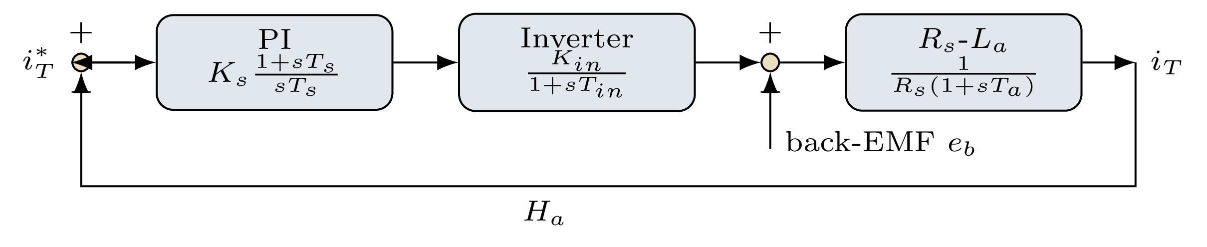
Current Controller Design
{Current Controller Design — Pole-Zero Cancellation}Inner Current Loop Structure

PI Current Controller
\[
G_c(s) = K_s\,\frac{1 + sT_s}{sT_s}
\]
- PI zero placed at \(s = -1/T_s\)
- Set \(T_s = T_a = L_a/R_s\) to cancel the plant pole
- Pole-zero cancellation leaves a pure integrator in the open loop, ensuring zero steady-state error
Closed Current-Loop Transfer Function
After pole cancellation (\(T_s = T_a\)):
\[
G_i(s) = \frac{K_i}{1 + sT_i}
\]
\[
K_i = \frac{K_s\,K_{in}\,T_a}{T_{ar}}, \quad
T_i = T_1
\]
Model Reduction
The higher-order current loop is reduced to a first-order approximation — essential for systematic speed-controller synthesis.Complete Current Loop Transfer Function
{Complete Current Loop — Exact and Simplified Forms}Open-Loop Transfer Function (Exact)
\[
G_i(s) = \frac{K_s\,K_{in}\,T_s\,(1+sT_m)}{T_{ar}\,T_m\,(1+sT_1)(1+sT_2)}
\]
\[
G_i(s) \approx \frac{K_i}{1 + sT_i}, \quad
K_i = \frac{K_s\,K_{in}\,T_1}{T_{ar}}
\]
Validation of Approximation
Bode plot comparison between exact and simplified current loop:
- Gain discrepancy at high frequency (acceptable)
- Phase responses almost identical in the frequency range of interest
- Both models cross 0\,dB at the same \(\omega_c\)
- Simplified model sufficient for speed-loop design
Speed Loop Design - Symmetric Optimum
Speed Loop Architecture
{Speed Loop Architecture and Mechanical Subsystem}Speed Loop Structure
Mechanical Subsystem Transfer Function
\[
G_m(s) = \frac{K_m}{s(1 + sT_m)} = \frac{P/(2J)}{s\!\left(1+s\tfrac{B}{J}\right)}
\]
\[
T_m = J/B \quad\text{(mechanical time constant)}
\]
Speed-Loop Open-Loop Function
For the simplified model (first-order current loop):
\[
G_f(s) = \frac{K_m\,K_s\,(1+sT_s)}{s\,T_s\cdot s\,T_m\cdot
\tfrac{1}{K_i}(1+sT_i)(1+sT_\omega)}
\]
Symmetric Optimum Design
{Symmetric Optimum — Concept and Design Procedure}What is the Symmetric Optimum?
The symmetric optimum is a frequency-domain design criterion
that maximises the phase margin at the gain crossover frequency for
a given closed-loop bandwidth, while ensuring zero steady-state error
to step disturbances.
Design Formulas
For a plant \(G_p(s) = K_p/[s(1+s\tau)]\), the symmetric
optimum yields PI parameters:
\[
T_s = a^2\tau, \quad
K_s = \frac{1}{2a\,K_p\,\tau} \quad (a \ge 2)
\]
- Crossover frequency: \(\omega_c = 1/(a\tau)\)
- Phase margin with \(a=2\): \(\varphi_m \approx 36°\)
- Phase margin with \(a=3\): \(\varphi_m \approx 53°\) (recommended choice)
- Parameter \(a\) trades off bandwidth against stability margin
Why ``Symmetric''?
The Bode phase plot is symmetric about the crossover frequency \(\omega_c\):- The PI zero contributes equal phase lead below \(\omega_c\)
- The plant pole contributes equal phase lag above \(\omega_c\)
- This symmetry maximises the phase margin for a given crossover frequency
- Optimises disturbance rejection bandwidth
Speed-Loop Transfer Functions
{Speed-Loop Transfer Functions — Exact and Simplified}Closed-Loop Speed Transfer Functions
Exact speed-loop transfer function:
\[
G_{\omega e}(s) = \frac{\omega_r(s)}{\omega_r^*(s)}
= \frac{G_{\omega f}(s)}{1 + G_{\omega f}(s)\,G_\omega(s)}
\]
\[
G_{\omega s}(s) = \frac{G_f(s)}{1 + G_f(s)\,G_\omega(s)}
\]
\[
G_{\omega ss}(s) = \frac{G_{\omega s}(s)}{1+sT_s}
\]
Verification
Bode plot comparison confirms:
- Gain difference at high frequencies (higher-order terms)
- Phase responses nearly identical in the bandwidth of interest
- Crossover at the same \(\omega_c\)
- Simplified model is adequate for controller synthesis
Reference Pre-filter
{Reference Pre-filter and Step Response Characteristics}Reference Pre-filter
A first-order low-pass filter is added to the speed reference
to eliminate the PI-zero overshoot in the tracking response:
\[
F(s) = \frac{1}{1 + sT_f}, \quad T_f = T_s
\]
- Cancels the PI zero in the closed-loop numerator
- Converts the tracking response to a well-damped second-order Butterworth-like shape
- The disturbance rejection response is unchanged (pre-filter is not in the disturbance path)
Step Response Characteristics (\(a=3\))
- Rise time: \(\approx 3/\omega_c\)
- Overshoot: \(< 5\%\) (with pre-filter)
- Settling time: \(\approx 8/\omega_c\)
- Load step recovery: \(\approx T_m\)
Design Recommendation
Always include the reference pre-filter when the symmetric optimum is used for speed-loop design — it transforms a fast but oscillatory response into a well-damped one at no cost to disturbance rejection.Complete Drive Architecture
{Complete Indirect Vector-Controlled Drive with Speed Controller}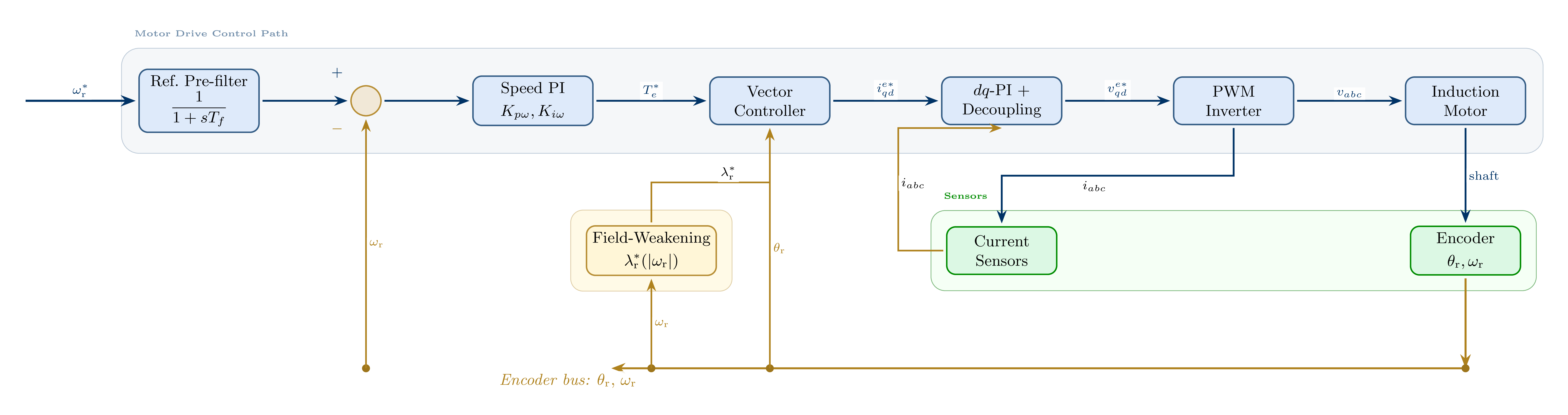 \caption{Complete block diagram of the indirect vector-controlled induction
motor drive with cascade speed and current controllers}
\caption{Complete block diagram of the indirect vector-controlled induction
motor drive with cascade speed and current controllers}
Design Procedure
- Current loop: design PI gains using pole-zero cancellation (\(T_s = T_a\), \(K_s\) from bandwidth specification)
- Model reduction: reduce current loop to first-order \(K_i/(1+sT_i)\)
- Speed loop plant: combine reduced current loop, mechanical subsystem, and speed sensor model
- Symmetric optimum: apply design formulas with \(a = 3\) (recommended)
- Reference pre-filter: set \(T_f = T_s\)
- Verification: simulate step response and load disturbance rejection; compare exact vs.\ simplified
Summary of Parameter Expressions
\begin{align*}
T_a &= L_a / R_s &&\text{(stator transient TC)} \\
T_m &= J / B &&\text{(mechanical TC)} \\
T_{ar} &= T_a + T_{in}&&\text{(combined TC)} \\
T_i &= T_1 &&\text{(current loop TC)} \\
T_s &= a^2 T_i &&\text{(speed PI zero TC)} \\
K_{\omega s} &= \frac{1}{2a\,K_m\,K_i\,H_\omega\,T_i} &&
\end{align*}
Typical Values with \(a = 3\)
Phase margin \(\approx 53°\)\\ Bandwidth \(\omega_c = 1/(3T_i)\)\\ Good disturbance rejection and reference trackingSummary
{Summary — Lecture 8 and Course Overview}Key Results of Lecture 8
- The torque channel of the vector-controlled IM is modelled as a first-order \(R_s\)-\(L_a\) plant — identical in form to a DC motor armature circuit
- Inner PI current controller with pole-zero cancellation simplifies to \(K_i/(1+sT_i)\)
- Speed loop designed via symmetric optimum maximises phase margin for a given bandwidth
- Reference pre-filter \(1/(1+sT_s)\) eliminates PI-zero overshoot without affecting disturbance rejection
- Complete cascade: reference filter \(\to\) speed PI \(\to\) vector controller \(\to\) current PI \(\to\) VSI \(\to\) IM
Course — Complete Overview
| cl@{}} Lecture | Topic | |
| 1 | Introduction \ | Principle |
| 2 | Direct Vector Control | |
| 3 | Indirect Vector Control | |
| 4 | Steady State \ | Dynamics |
| 5 | Parameter Sensitivity | |
| 6 | Parameter Compensation | |
| 7 | Flux-Weakening Operation | |
| 8 | Speed-Controller Design |
Course Take-Away
Vector control transforms the induction motor into a high-performance, independently-controllable flux-and-torque machine — enabling AC drives to surpass DC machines in precision, speed range, and robustness.