Need for Flux Weakening
Voltage Constraint Analysis
{Voltage Constraint and the Need for Flux Weakening}Inverter Voltage Limit
The stator voltage phasor magnitude is bounded by the inverter
DC-link voltage:
\[
V_s \le V_{s,\max} = \frac{V_{dc}}{\sqrt{3}}
\quad\text{(six-step limit)}
\]
\[
V_s \approx \omegas\sqrt{(\sigma\Ls\,\iqs)^2
+ \!\left(\sigma\Ls\,\ids + \tfrac{\Lm}{\Lr}\lambdar\right)^2}
\]
Flux-Weakening Law
Reduce the rotor flux inversely with synchronous speed:
\[
\lambdar^* \propto \frac{1}{\omegas}
\quad (\omegas > \omega_b)
\]
Constant-Power Characteristic
With \(\lambdar \propto 1/\omegas\) and \(\iT \approx\) const:\[
\Te \propto \lambdar\cdot\iT \propto \frac{1}{\omegas}
\]
\[
P = \Te\cdot\omegar \approx \text{const}
\]
Operating Regions
{Operating Regions of the Vector-Controlled Drive}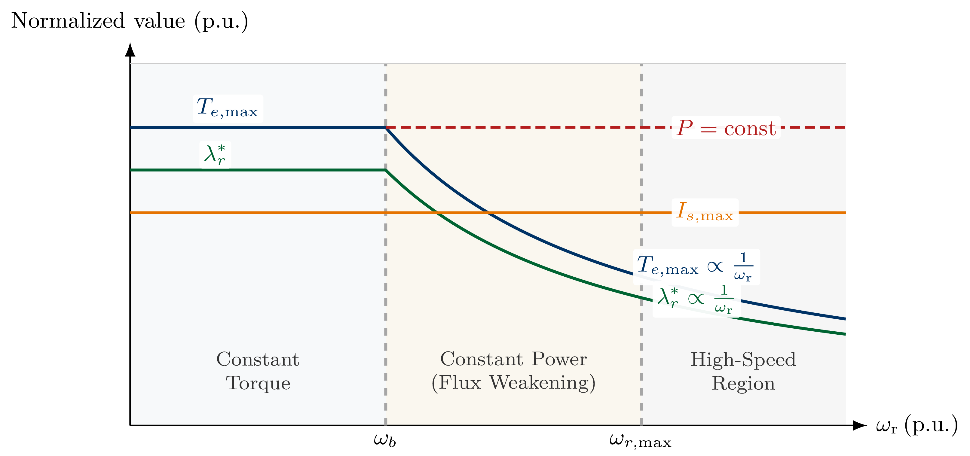 \caption{Torque-speed characteristic showing constant-torque,
constant-power, and high-speed flux-weakening regions
of the vector-controlled drive}
\caption{Torque-speed characteristic showing constant-torque,
constant-power, and high-speed flux-weakening regions
of the vector-controlled drive}
Stator-Flux-Linkage-Controlled Schemes
Normalised Voltage Equations
{Normalised Stator Voltage Equations in Flux Weakening}Stator Equations in Synchronous Frame (Normalised, Steady State)
Neglecting stator resistive drops and setting \(p = 0\):
\begin{align*}
v_{qsn}^e &\cong \omega_{sn}\,\lambda_{dsn}^e \\[4pt]
v_{dsn}^e &\cong -\omega_{sn}\,\lambda_{qsn}^e
\end{align*}
\[
v_{sn} = \omega_{sn}\sqrt{(\lambda_{qsn}^e)^2 + (\lambda_{dsn}^e)^2}
= \omega_{sn}\,\lambda_{sn}
\]
Stator Flux in Flux Weakening
\[
\lambda_{sn} = \frac{v_{sn}}{\omega_{sn}}
\]
Key Result for Stator-Flux Control
With the stator flux aligned to the \(d\)-axis (\(\lambda_{qsn}^e = 0\)):- Torque: \(T_{en} = i_{qsn}^e\,\lambda_{sn}\)
- Air-gap power: \(P_{an} = v_{sn}\,i_{qsn}^e\)
- If \(i_{qsn}^e = \) const and \(v_{sn} = \) const, then \(P_{an} = \) const
Air-Gap Power in the Flux-Weakening Region
{Constant Air-Gap Power in the Flux-Weakening Region}Air-Gap Power Derivation
The normalised air-gap power:
\[
P_{an} = T_{en}\cdot\omega_{sn}
= i_{qsn}^e\,\lambda_{sn}\,\omega_{sn}
= i_{qsn}^e\,v_{sn}^e
\]
\[
P_{an} = v_{sn}\,i_{qsn}^e = \text{const}
\quad \text{if } i_{qsn}^e = \text{const}
\]
- Maintaining \(i_{qsn}^e\) constant maintains constant power
- Achieved by holding \(I_{s,\max}\) and adjusting flux such that \(i_{qsn}^e = \iT\) remains at its rated value
Stator-Flux Weakening Algorithm
- Monitor \(|v_s|\) (measured or estimated from model)
- When \(|v_s| \to V_{s,\max}\): initiate flux weakening
- Set \(\lambdas^* = V_{s,\max}/\omega_s\)
- Hold \(q\)-axis current at its limiter value
- \(d\)-axis current adjusts automatically via flux controller
- Speed range limited only by the \(\iT\) capability
Rotor-Flux-Linkage-Controlled Schemes
Rotor-Flux Weakening Strategy
{Rotor-Flux Weakening in Indirect Vector Control}Voltage Constraint in the Rotor-Flux Frame
In the indirect vector-control scheme with rotor flux aligned
to the \(d\)-axis:
\begin{align*}
v\qs &\approx \omegas\!\left(\sigma\Ls\,\ids
+ \tfrac{\Lm}{\Lr}\lambdar\right)\\[4pt]
v\ds &\approx -\omegas\,\sigma\Ls\,\iqs
\end{align*}
Flux-Weakening Law
\[
\lambdar^* = \frac{V_{s,\max}}{\omegas}\cdot\frac{\Lr}{\Lm}
\quad (\omegas > \omega_b)
\]
\[
\ifld^* = \frac{\lambdar^*}{\Lm^*} = \frac{V_{s,\max}}{\omegas\,\Lm^*}
\]
Implementation in Indirect VC
- A voltage limiter detects when the VSI approaches saturation
- Alternatively: an open-loop schedule \(\lambdar^* = f(1/\omegas)\) is pre-programmed
- The slip-speed command during flux weakening becomes:
where \(\ifld^*(t)\) is now time-varying\[ \omegasl^* = \frac{\iT^*}{\Tr^*\,\ifld^*(t)} \]
- The lead compensator in \(\ifld^*\) ensures fast flux response during flux-change transients
Torque Capability and Optimisation
{Torque Capability and Optimal Flux in the Flux-Weakening Region}Maximum Torque vs.\ Speed
With stator current limit \(I_{s,\max}\) and voltage limit \(V_{s,\max}\):
\[
T_{e,\max}(\omegas) = K_{te}\,\lambdar(\omegas)\,I_{T,\max}
\]
\[
\lambdar(\omegas) = \frac{V_{s,\max}}{\omegas}\cdot\frac{\Lr}{\Lm},
\quad
I_{T,\max} = \sqrt{I_{s,\max}^2 - \ifld^{*2}}
\]
Optimal Flux for Maximum Torque
The flux value maximising torque at a given speed is found from:\[
\frac{\partial \Te}{\partial \lambdar}\bigg|_{I_s = I_{s,\max}} = 0
\]
\[
\lambdar^{\mathrm{opt}} = \frac{\Lm\,I_{s,\max}}{\sqrt{2}}
\]
\[
\ifld = \iT = \frac{I_{s,\max}}{\sqrt{2}}
\]
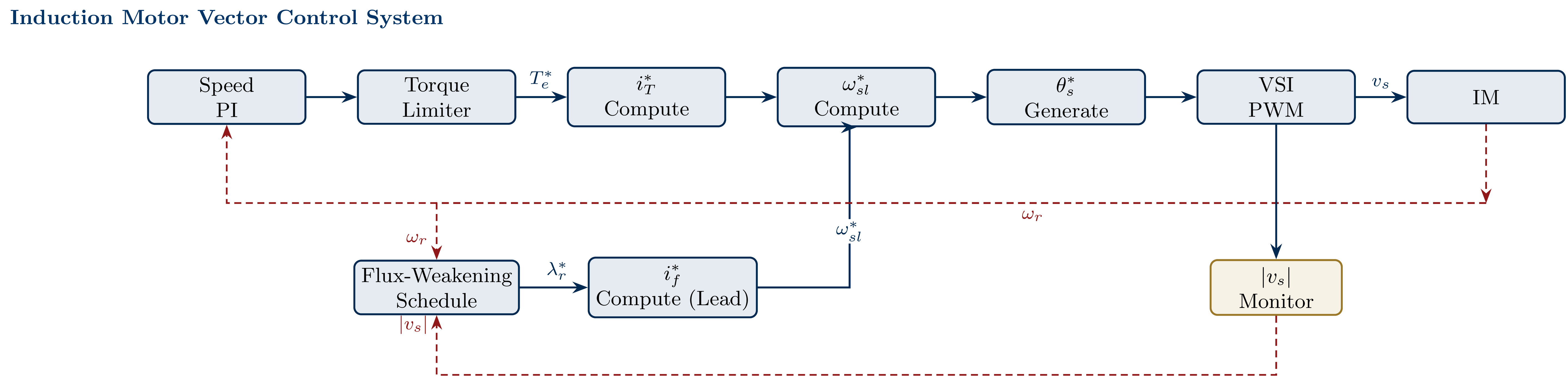 \caption{Block diagram of the practical flux-weakening controller integrated
with the indirect vector control scheme}
\caption{Block diagram of the practical flux-weakening controller integrated
with the indirect vector control scheme}
- Flux-weakening is triggered when measured \(|v_s| \to V_{s,\max}\)
- The lead compensator \((1 + s\Tr^*)\) in \(\ifld^*\) ensures fast flux response during the constant-to-weakening transition
Summary
{Summary — Lecture 7}Key Concepts
- Flux weakening extends the speed range above \(\omega_b\) by reducing \(\lambdar\) in proportion to \(1/\omegas\), keeping \(V_s \le V_{s,\max}\)
- Approximately constant output power is maintained if the torque-producing current is held constant
- Stator-flux scheme (direct VC): flux reduced to \(\lambdas^* = V_{s,\max}/\omegas\); elegant constant-power law
- Rotor-flux scheme (indirect VC): flux reduced via updated \(\ifld^*\) schedule; more sensitive to \(\Rr\) mismatch
- Optimal flux for maximum torque: \(\ifld = \iT = I_{s,\max}/\sqrt{2}\)
Applications Demanding Flux Weakening
- Electric vehicle traction drives (2–4\(\times\) base speed)
- Machine tool spindle drives (up to 10\(\times\) base speed)
- Centrifuges and high-speed blowers
- Wind turbine generators (variable wind speed)
Important Reminder
Flux weakening in indirect VC increases the commanded slip speed, amplifying sensitivity to \(\Rr\) mismatch. Robust parameter compensation (Lecture~6) is therefore even more critical in the flux-weakening region.