Phase-Controlled Induction-Motor Drives — Introduction & Steady-State Analysis

SECTION 01

Four-Lecture Series — Road Map

Lecture Plan

L1 [This lecture] — Speed-control overview · SCR power circuit · reversible controller · induction motor power flow · waveform analysis · steady-state analysis · torque stability · torque–speed characteristics
L2 — Load interaction · thermal limits · power factor · closed-loop cascade control · efficiency · applications
L3 — Slip-energy recovery (SER): circuit, equivalent model, \(T_e\)–\(I_{dc}\) analogy, harmonics, supply-side distortion, ratings, closed-loop control
L4 — Static Scherbius drive · supersynchronous operation · industrial and wind (DFIG) applications · reactive power control · unified comparative summary

Learning Objectives — Lecture 6A

After this lecture you should be able to:

Identify the three approaches to IM speed control and their trade-offs
Explain air-gap power partition and the \((1-s)\) efficiency ceiling
Describe SCR voltage waveforms for varying firing angle \(\alpha\)
Explain the role of firing angle \(\alpha\) in a phase-controlled drive
Describe the reversible controller and its operational quadrants
State the torque stability criterion and identify the stable operating region
Derive conduction angle \(\beta\) from the transcendental equation
Compute normalised torque–speed characteristics for a given \(\alpha\)

SECTION 02

Speed Control of Induction Motors — Overview

Fundamental Speed Equation

Speed is controlled by varying pole count \(P\), supply frequency \(f_s\), or slip \(s\):

\[\omega_{m} = \frac{4\pi f_s}{P}(1-s) \qquad\Longrightarrow\qquad \omega_{m}\ \text{controlled by varying}\ \underbrace{P}_{\text{pole count}},\quad \underbrace{f_s}_{\text{supply freq.}},\quad\text{or}\quad \underbrace{s}_{\text{slip}}\]

Pole Changing

Rewire stator windings to change pole count. Provides discrete speed steps (2–3 levels) with no continuous control. Rarely used in modern drives.

Slip (Stator-Voltage) Control

Vary \(V_s\) via SCRs. Efficiency ceiling: \(\eta \leq (1-s)\). Simple circuit; poor efficiency at low speed.

Focus of Lectures 1–2.

Frequency Control

Variable-frequency PWM inverter. High efficiency at all speeds. Dominant modern approach (V/f, FOC, DTC).

🎯

Series Focus

Phase-Controlled (Slip-Based) Drives

This series focuses on phase-controlled drives — relevant for large wound-rotor machines and soft-starters.

SECTION 03

Power Flow in the Induction Motor — The Air-Gap Partition

Complete Power Balance (Per-Phase, Referred to Stator)

\[P_{\text{in}} = 3\,V_s I_s \cos\phi_s \quad\text{(electrical input)}\]

\[P_{s,\text{cu}} = 3\,I_s^2 R_s \quad\text{(stator copper loss)}\]

\[P_{ag} = P_{\text{in}} - P_{s,\text{cu}} - P_{\text{core}} \quad\text{(air-gap power)}\]

Air-gap power splits with slip:

\[\underbrace{P_{ag}}_{\text{air-gap power}} = \underbrace{s\,P_{ag}}_{P_{r,\text{cu}}\ (\text{rotor copper})} + \underbrace{(1-s)\,P_{ag}}_{P_{\text{mech}}\ (\text{shaft power})}\]

Torque–air-gap power link:

\[T_e = \frac{P_{ag}}{\omega_s} \qquad\Longrightarrow\qquad P_{\text{mech}} = T_e\,\omega_r\]

where \(\omega_s\) is the synchronous mechanical speed.

Fundamental Efficiency Ceiling

Rotor copper loss \(= s\,P_{ag}\) rises linearly with slip. Even with ideal stator and zero core losses:

\[\eta \leq \frac{P_{\text{mech}}}{P_{ag}} = \frac{(1-s)P_{ag}}{P_{ag}} = \boxed{1 - s}\]

Reducing speed means higher slip; efficiency falls in direct proportion.

Why this matters for drives:

Resistor control: \(sP_{ag}\) dissipated in external resistors.
Phase (SCR) control: \(sP_{ag}\) dissipated in the rotor only.
SER (Lecture 3): \(sP_{ag}\) is recovered and returned to the supply \(\Rightarrow\) \(\eta \gg (1-s)\).

SECTION 04

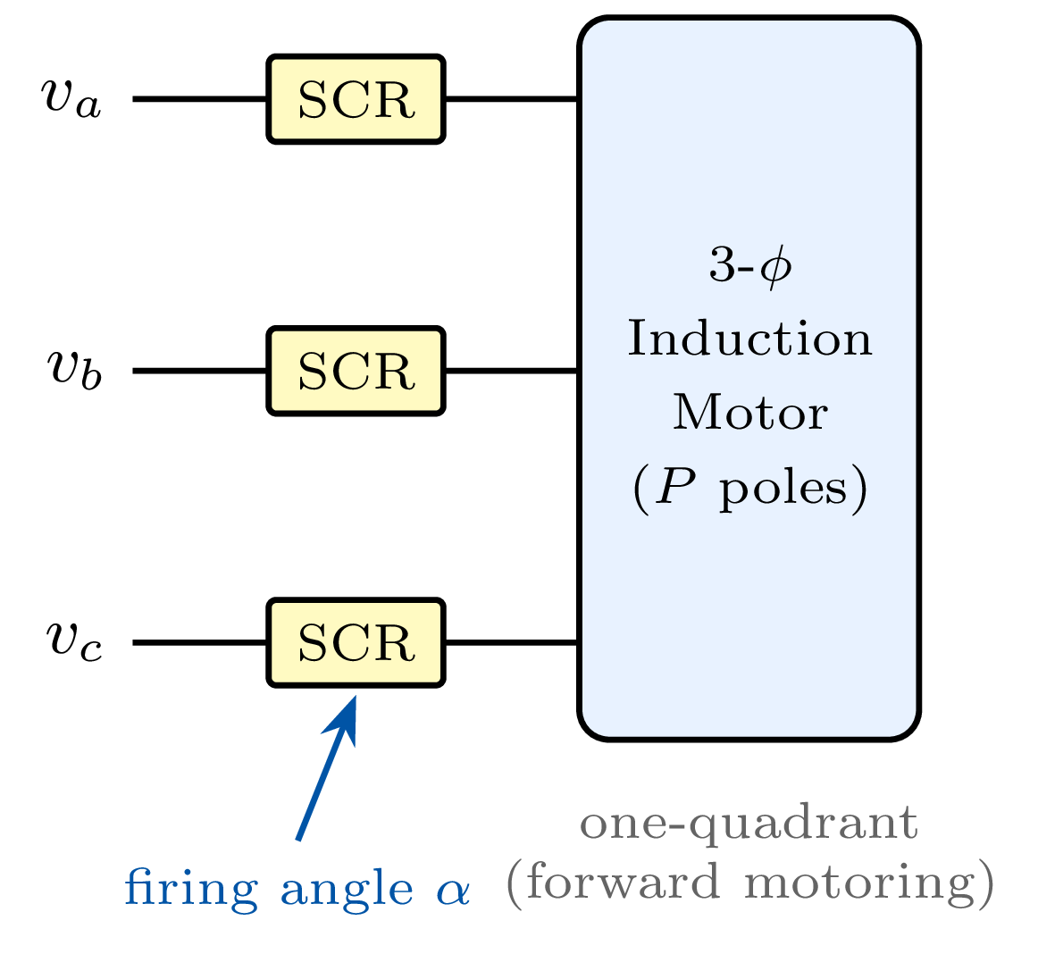
Power Circuit of the Phase-Controlled IM Drive

Operating Principle and Reversible Controller

Operating principle:

Power switches (SCR or TRIAC) placed in series with each stator phase.
Each gate pulse is delayed by firing angle \(\alpha\) with respect to the natural commutation point of the phase voltage.
For \(\alpha > \phi\) (motor power-factor angle), the switch conducts for a partial conduction angle \(\beta < 180°\), reducing the rms stator voltage.
Three back-to-back SCR pairs (or TRIACs) control all three phases simultaneously.

Reversible controller:

Two anti-parallel SCR groups allow Quadrants I and III operation.
A dead-time blanking interval prevents simultaneous conduction (shoot-through protection).

SCR phase-controlled induction motor drive power circuit showing three back-to-back SCR pairs in series with the three stator phases and a reversible anti-parallel controller — Phase-controlled IM drive: power circuit with anti-parallel SCR groups for bidirectional operation

SECTION 05

Waveform Analysis — Steady-State via Thévenin Equivalent

Thévenin Equivalent and Instantaneous Stator Current

Thévenin equivalent (referred to stator):

\[R_{eq} = R_s + \frac{(R_r/s)\,X_m^2}{(R_r/s)^2+(X_r+X_m)^2}\]

\[X_{eq} = X_s + \frac{X_m\bigl[(R_r/s)^2+X_m(X_r+X_m)\bigr]}{(R_r/s)^2+(X_r+X_m)^2}\]

\[Z_{eq}=\sqrt{R_{eq}^2+X_{eq}^2},\qquad \phi = \arctan\!\left(\frac{X_{eq}}{R_{eq}}\right)\]

Instantaneous stator current (phase \(a\)):

\[i_s(\omega t)=\frac{V_m}{Z_{eq}} \Bigl[\sin(\omega t-\phi) -\sin(\alpha-\phi)\,e^{-(\omega t-\alpha)/\tan\phi}\Bigr]\]

valid for \(\omega t \in [\alpha,\;\alpha+\beta]\), where \(V_m=\sqrt{2}\,V_s\) is the peak phase voltage.

SECTION 06

Conduction Angle and Normalised Stator Voltage

Conduction-Angle Transcendental Equation

Setting \(i_s(\alpha+\beta)=0\):

\[\sin(\alpha+\beta-\phi) =\sin(\alpha-\phi)\,e^{-\beta/\tan\phi}\]

Transcendental in \(\beta\); solved iteratively by Newton–Raphson.

Full Conduction (\(\alpha \leq \phi\))

Full conduction (\(\beta = 180°\)); voltage is uncontrolled.

Partial Conduction (\(\alpha > \phi\))

Partial conduction (\(\beta < 180°\)); voltage is reduced.

Normalised rms stator voltage:

\[V_{1n} = \sqrt{\frac{1}{\pi} \Bigl[\beta+\sin 2\alpha-\sin(2\alpha+2\beta)\Bigr]} \;\text{p.u.}\]

(all angles in radians; \(\beta\) is the conduction angle per half-cycle)

Conduction Angle vs. Firing Angle

Graph of conduction angle beta versus firing angle alpha showing flat region at 180 degrees for alpha less than phi, then decreasing region for different motor power-factor angles phi — Conduction angle \(\beta\) vs. firing angle \(\alpha\) for different motor power-factor angles \(\phi\)

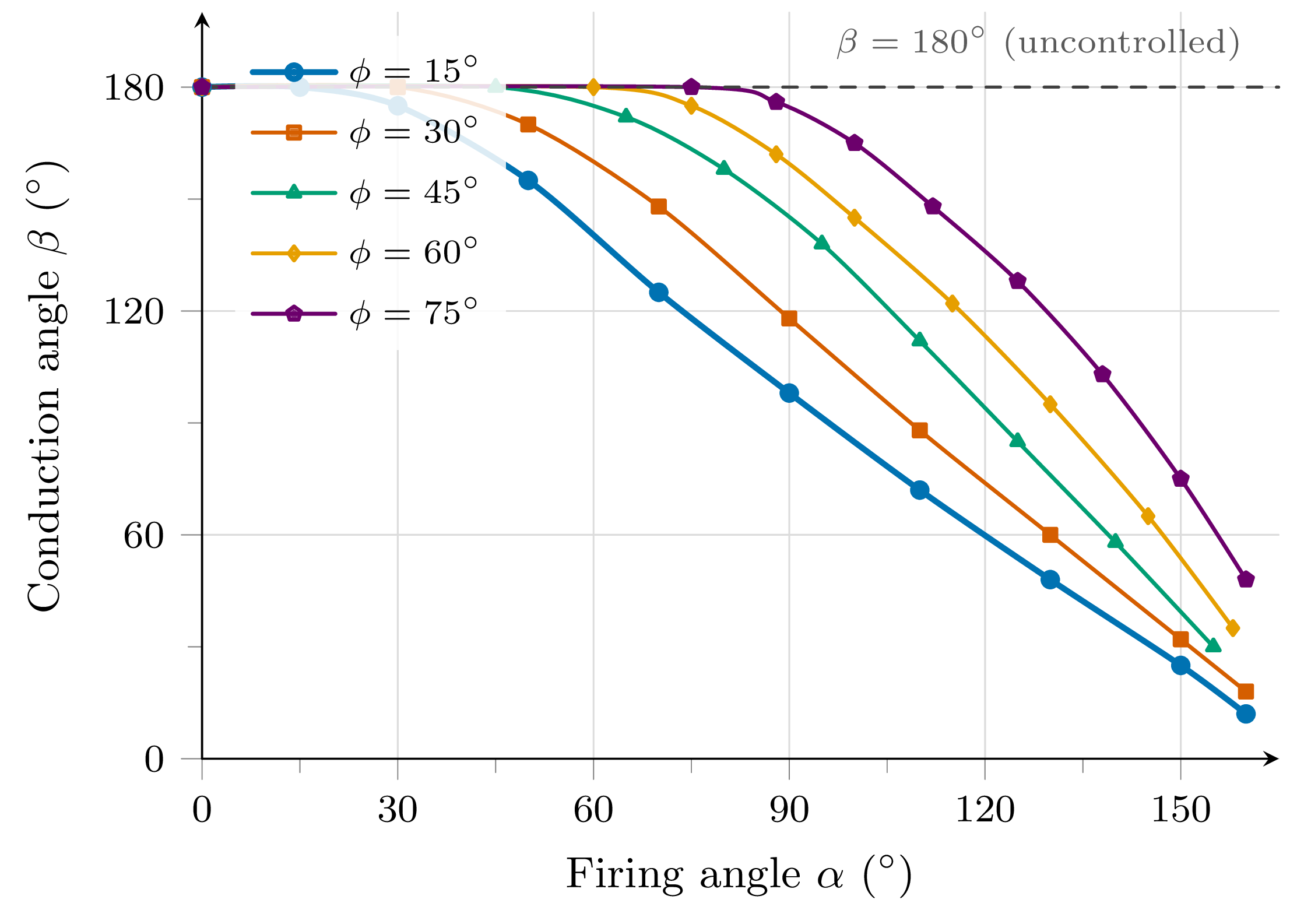
Key observations:

Flat region (\(\beta = 180°\)): no control effect; motor sees full voltage. Control begins only for \(\alpha > \phi\).
Decreasing region: increasing \(\alpha\) reduces \(\beta\), hence \(V_{1n}\) and electromagnetic torque.
A more inductive motor (larger \(\phi\)) requires a higher \(\alpha\) before voltage reduction starts.
As \(\alpha \to 180°\), \(\beta \to 0\): motor is effectively de-energised.
For a given \(\alpha\), \(\beta\) also depends on slip (via \(\phi\)); curves must be recalculated at each operating point.

Model validity: Analytical model is valid for \(\alpha \lesssim 135°\). Beyond this, harmonic distortion is severe and a full \(d\)–\(q\) dynamic simulation is required.

SECTION 07

Torque Stability Criterion

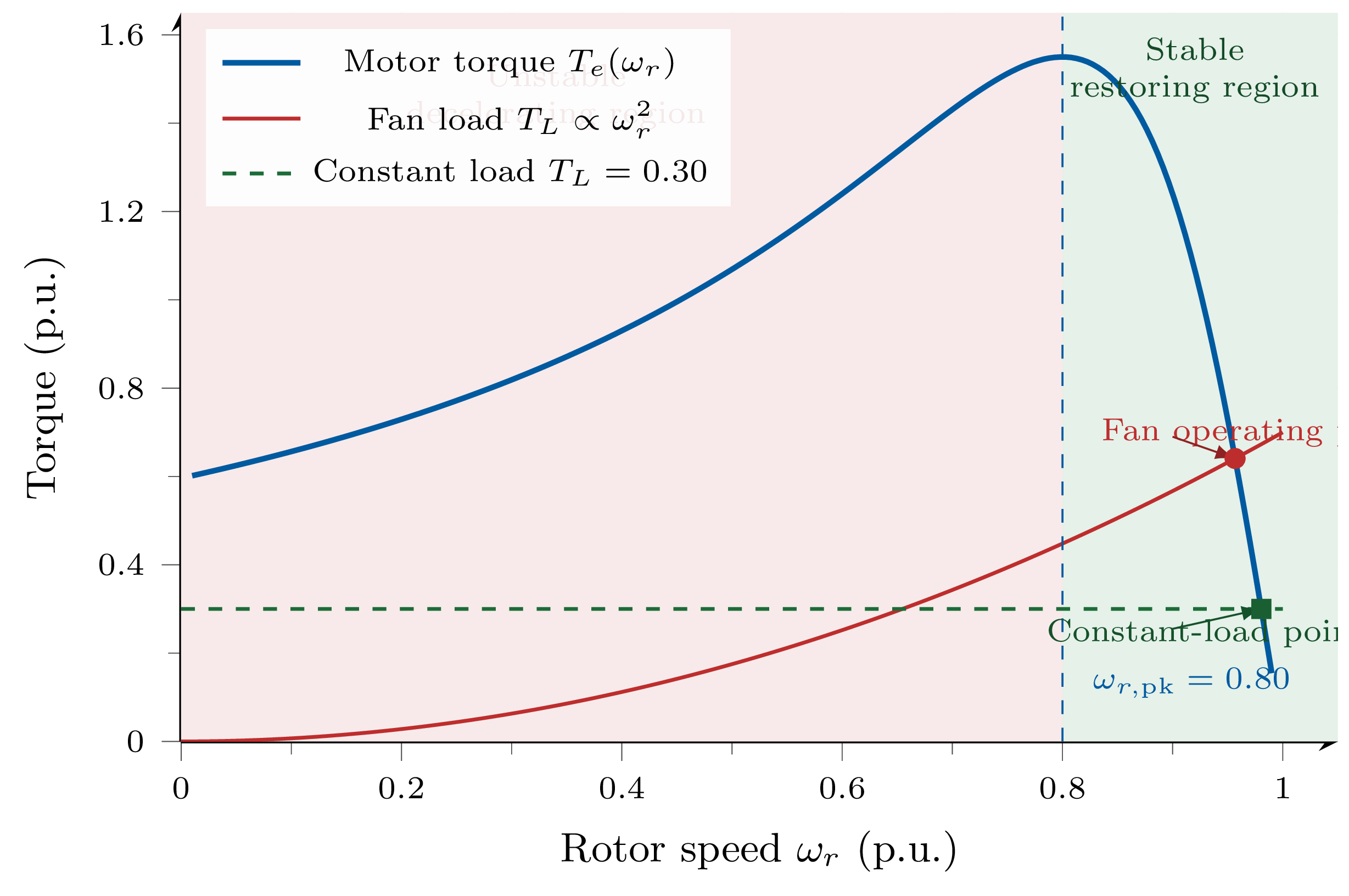
Stability Condition for Steady-State Operation

Torque-speed characteristics of induction motor showing stable operating region on the low-slip side and open-loop unstable region on the high-slip side of peak torque — Torque–speed characteristics showing stable and unstable operating regions

At the load–torque intersection, operation is stable if and only if:

\[\left.\frac{dT_e}{d\omega_r}\right|_{\text{OP}} < \left.\frac{dT_L}{d\omega_r}\right|_{\text{OP}}\]

Right of peak torque (\(s < s_\text{pk}\), low slip): \(T_e\) falls as speed rises; the intersection with the load curve is on the stable side.
Left of peak torque (\(s > s_\text{pk}\), high slip): \(T_e\) rises as speed rises; any upward perturbation leads to runaway — this region is open-loop unstable.

Implication for phase-controlled drives: Reducing \(V_s\) scales the entire \(T_e\)–\(\omega_r\) family downward by \(V_s^2\). If the load torque exceeds the new peak electromagnetic torque, the motor stalls. Closed-loop current limiting prevents this.

NEMA D advantage: High \(R_r\) moves peak torque toward standstill, enlarging the stable operating region.

SECTION 08

Normalised Torque–Speed Characteristics

Normalised Torque Expression and 5-Step Computation

Family of normalised torque-slip curves for different SCR firing angles alpha showing the curves shifted downward and narrowed as alpha increases — Normalised torque–slip curves for different firing angles \(\alpha\)

\[T_{en} = \frac{V_{1n}^2\,(R_{rn}/s)}{(R_{rn}/s)^2 + X_{rn}^2}\;\text{p.u.}\]

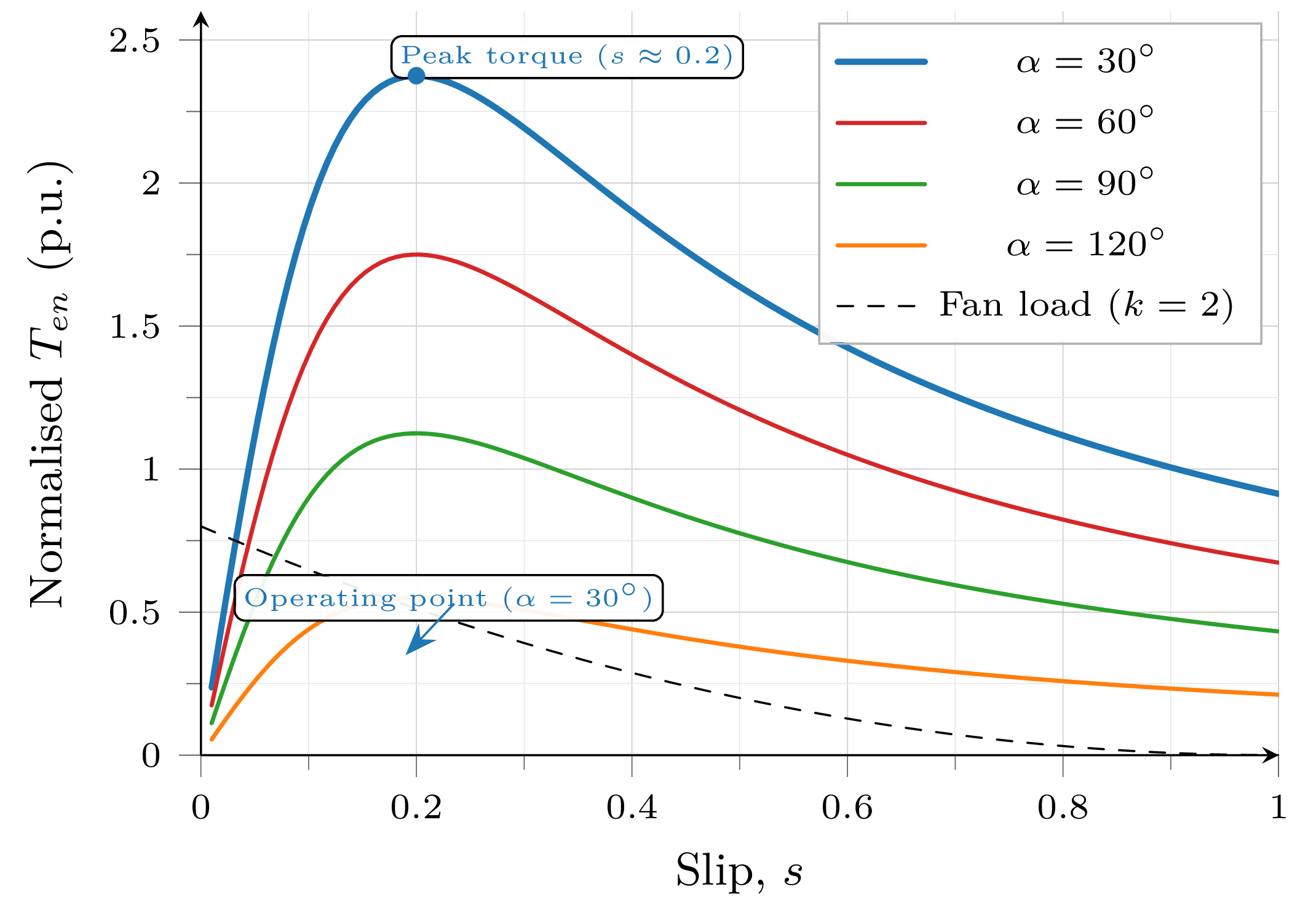
where all quantities are in per unit on a consistent motor base.

Computation procedure:

Choose slip \(s\) \(\Rightarrow\) compute \(Z_{eq},\,\phi\).
Given \((\alpha,\phi)\) \(\Rightarrow\) solve for \(\beta\) (Newton–Raphson).
Evaluate \(V_{1n}\) from the rms-voltage formula.
Compute \(T_{en}\).
Repeat for the full range of \(s\) and \(\alpha\).

Open-loop speed limitation: For a fan load (\(T_L \propto \omega_r^2\)) the open-loop speed variation spans only \(\approx 6\,\%\) of rated speed. Closed-loop control (Lecture 2) is essential for a useful speed range.

SECTION 09

Summary and Preview

What We Covered

Three IM speed-control strategies; phase control is slip-based with \(\eta \leq (1{-}s)\).
Air-gap power partition: \(P_{ag}= P_{r,cu}+ P_{\text{mech}}\); rotor copper loss \(= s\,P_{ag}\).
SCR waveforms: non-sinusoidal for \(\alpha>\phi\); harmonics increase with \(\alpha\).
Firing angle \(\alpha\) reduces rms stator voltage; control only for \(\alpha > \phi\).
Reversible drive: anti-parallel switch groups with dead-time blanking give Quadrants I and III operation.
Stability criterion: \(dT_e/d\omega_r < dT_L/d\omega_r\) at the operating point.
Conduction angle \(\beta\): transcendental equation; solved by Newton–Raphson.
Normalised torque–speed family via the 5-step procedure.

Preview — Lecture 6B

Load interaction: rotor and stator current profiles vs. speed for \(k = 0, 1, 2\) loads
Thermal constraints: peak current location and safe operating band
Input power factor and reactive power consumption of the phase-controlled drive
Closed-loop cascade controller: inner current loop + outer speed PI
Efficiency: phase control vs. external resistance
Applications and motivation for slip-energy recovery