Lecture 5D: Starting Methods & Speed Control | Polyphase Induction Machines

RECAP

Summary of Lectures 5A–5C

✓Lectures 5A and 5B

Construction, rotating magnetic field, slip s, operating modes
Per-phase equivalent circuit; R_r′/s power split
P_ag:P_r,Cu:P_conv = 1:s:(1−s)
T_em = P_ag/ω_s

✓Lecture 5C

Torque-slip equation via Thévenin equivalent
T_max is independent of R_r′; s_max ∝ R_r′
NEMA design classes A, B, C, D
DC Resistance / No-load / Locked-rotor tests

The Starting Problem — Key Numbers

I_start = 5–7 × I_rated
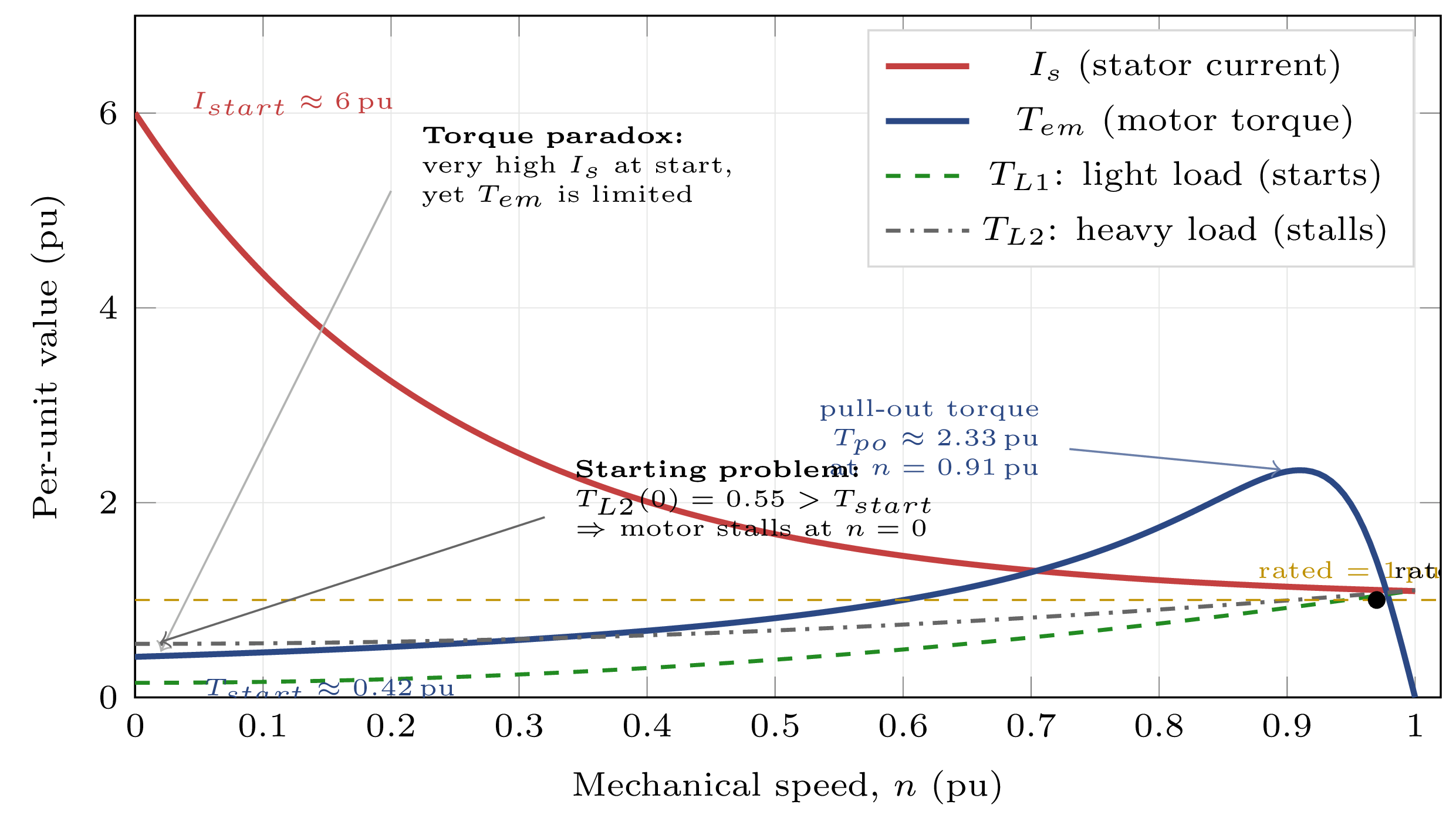
T_start ≈ (0.5–1.5) T_rated

High inrush current with only moderate torque — both issues require engineering solutions.

SECTION 01

The Starting Problem — Root Cause

System-Level Consequences of High I_start

Supply voltage dip: ΔV ∝ Z_source · I_start
Can cause a 10–20% dip for large motors
Trips sensitive equipment on the same feeder
Thermal stress: I²t constraint on stator windings

⚖️The Torque Paradox

Reducing voltage to limit current hurts torque even more, because T_em ∝ V_s²:

Voltage Reduction	Torque Reduction
10%	19%
33% (Y-Δ method)	56%

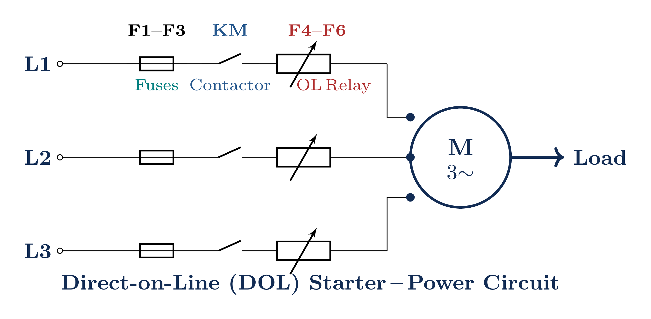
Graph illustrating the torque paradox in induction motor starting, showing disproportionate torque reduction versus current reduction — Fig. 1 — The torque paradox: T_em ∝ V_s² means voltage reduction hurts torque more than it limits current.

SECTION 02

Method 1 — Direct-On-Line (DOL) Starting

⚡Performance Summary

Starting current	5–7× I_rated
Starting torque	100% of DOL
Cost	Lowest
Complexity	Minimal

Advantages

Maximum available starting torque
Fastest motor acceleration
Simple: one contactor + overload relay only
Reliable, low maintenance

Limitations

Severe voltage dip on supply bus
Mechanical shock to couplings & gearboxes
High I²t thermal stress on windings
Unsuitable for weak supply grids

Direct-on-line starting circuit diagram showing a single contactor connecting the induction motor directly to the three-phase supply — Fig. 2 — DOL starting circuit: one main contactor + thermal overload relay.

📋Application Guide

P < 10 HP — generally acceptable
10 < P < 50 HP — case-by-case basis
P > 50 HP — usually not permitted

SECTION 03

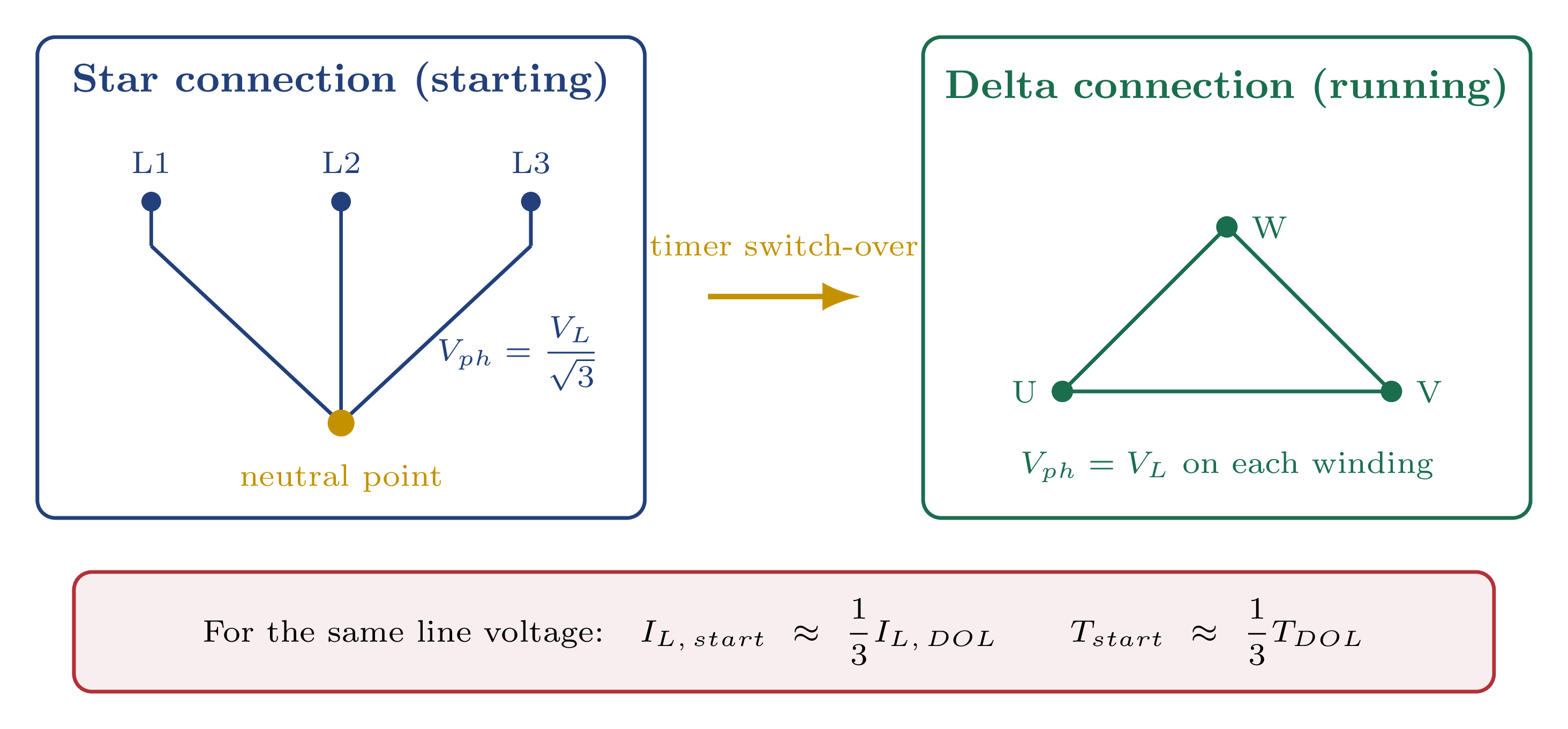
Method 2 — Star-Delta (Y-Δ) Starting

Motor designed for Δ at rated voltage is first connected in Y (phase voltage reduced by 1/√3), then switched to Δ at approximately 70–80% speed.

The 1/3 Rule — Derivation

Phase voltage in Y: V_Y = V_L/√3
Phase voltage in Δ: V_Δ = V_L
Phase current in Y: I_Y,ph = (V_L/√3) / Z_ph
Phase current in Δ: I_Δ,ph = V_L / Z_ph

I_Y,line = (1/3) · I_Δ,line
T_Y,start = (1/3) · T_Δ,start

What We Gain

Line current reduced to exactly 1/3 of DOL inrush
Starting torque reduced to exactly 1/3 of DOL torque
Low cost: three contactors, one timer
No additional power components

Key Limitations

Requires motor with 6 accessible terminals
Motor must be designed for Δ at rated line voltage
Y→Δ transition produces a second current transient
Torque reduction (1/3) may be too severe for high-inertia loads

Star-delta starting circuit diagram showing three contactors and a timer controlling the Y-to-Δ transition — Fig. 3 — Star-delta (Y-Δ) starting: three contactors reduce line current and torque to 1/3 of DOL values.

SECTION 04

Method 3 — Autotransformer Starting

A three-phase autotransformer steps the supply down to a selected tap during starting. Common taps: 50%, 65%, 80% of V_L. For tap ratio k (0 < k < 1):

Autotransformer Tap Ratio Equations

V_motor = k · V_L
I_line = k² · I_DOL
T_start = k² · T_DOL

Table 1 — Tap Comparison
Tap k	Motor Voltage	I_line/I_DOL	T/T_DOL
0.50	0.50 V_L	0.25	0.25
0.65	0.65 V_L	0.42	0.42
0.80	0.80 V_L	0.64	0.64

Advantages over Y-Δ

Multiple selectable taps — flexible for any load type
Works with Y- or Δ-connected motors (no 6-terminal requirement)
Better torque-per-supply-ampere ratio than Y-Δ
Suitable for high-inertia or heavily-loaded starts

Limitations

Transformer is bulky and relatively expensive
Transition transient still present at bypass
Typically chosen for P > 50 HP applications

SECTION 05

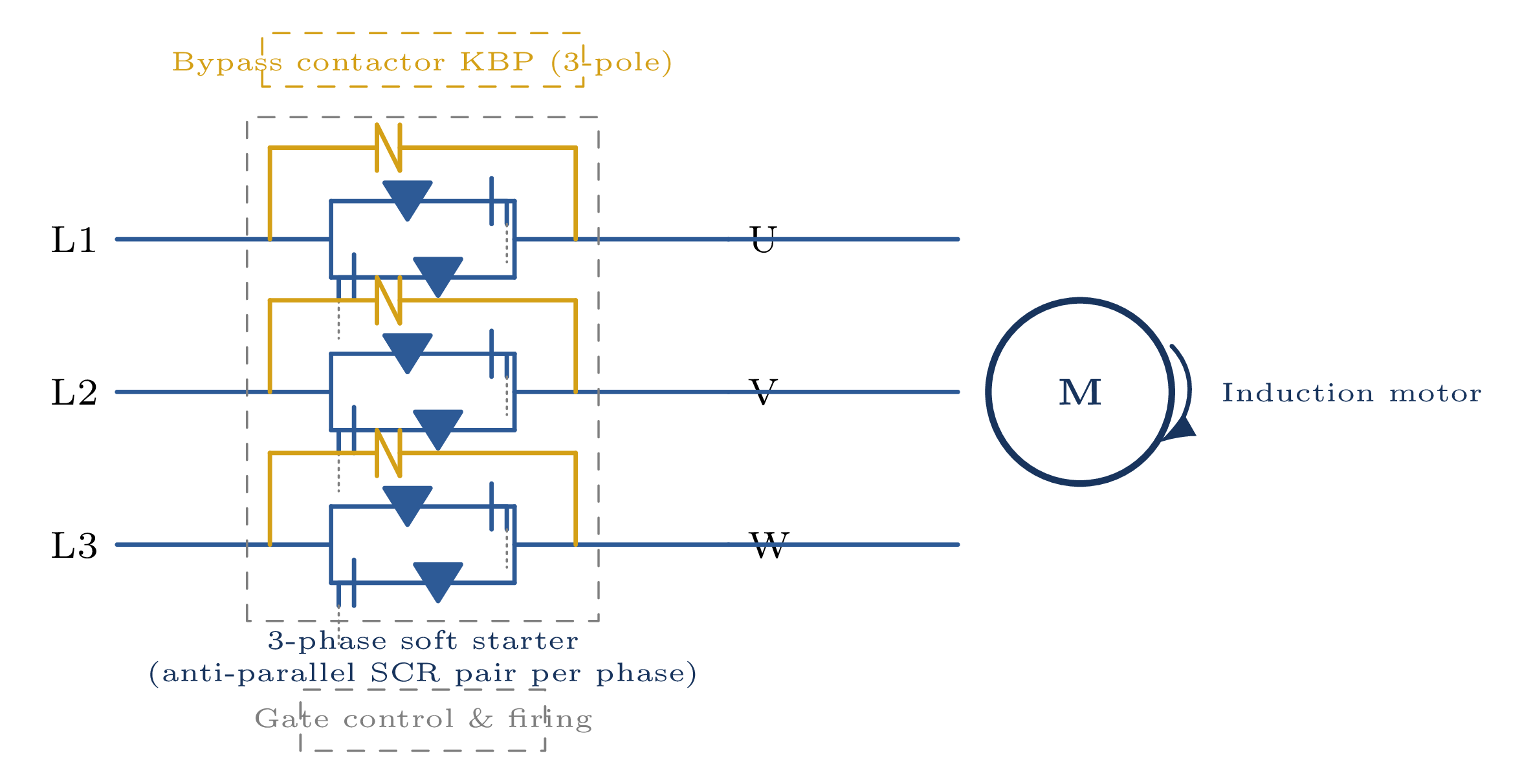
Method 4 — Soft Starters

Back-to-back SCR pairs in each phase control the firing angle α, progressively raising the RMS voltage from a low initial value to full line voltage over a programmable ramp time.

🎛️Control Modes

Voltage ramp — V rises linearly with time (simplest)
Current limit — I_s held constant during ramp (most common)
Torque control — V adjusted to match load profile
Kick-start — brief voltage pulse for high breakaway torque loads

Key Features

Smooth, jerk-free start — no transition transient
Soft stop (controlled deceleration) also available
Built-in protection: overload, phase loss, stall detection
Starting current only 2–4× I_rated (vs. 5–7× for DOL)

Soft starter circuit diagram showing back-to-back SCR thyristor pairs in each phase with a bypass contactor — Fig. 4 — Soft starter circuit: back-to-back SCRs ramp voltage from ~30% to 100%; bypass contactor closes at speed.

⚠️

Important Limitation

Soft starters cannot provide variable speed in steady state

Soft starters control voltage only — once running, the bypass contactor locks in full voltage. For continuous speed control, a VFD is required.

SECTION 06

Method 5 — Rotor Resistance Starting (Wound-Rotor)

External resistance inserted in the rotor circuit via slip rings and brushes. By choosing R_ext so that s_max = 1, we achieve T_start = T_max — maximum starting torque at near-rated current.

Modified Slip at Maximum Torque

s_max ≈ (R_r′ + R_ext) / (X_th + X_r′)

Torque-speed curves during wound-rotor resistance starting showing how progressive resistance removal maintains near-maximum torque — Fig. 5 — Wound-rotor starting: external R_ext set so s_max=1 ⇒ T_start=T_max.

Trade-off

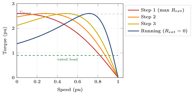
Starting: Excellent torque & controlled current
Running: Power wasted as heat in R_ext; P_loss = s · P_ag
Largely superseded by VFDs in modern installations

SECTION 07

Starting Methods — Complete Comparison

Table 2 — Starting Methods Comparison
Method	I_start/I_rated	T_start/T_DOL	Cost	Transient	Best For
DOL	5–7×	100%	Lowest	None	Small motors <10 HP
Star-Delta	1.7–2.3×	33%	Low	Surge at switchover	Light loads; 10–100 HP
Autotransformer (65%)	2.1–2.8×	42%	Medium	Surge at bypass	Heavy loads >50 HP
Soft Starter	2–4×	Variable	Med-High	None	Smooth start; all sizes
Rotor R_ext	≈1–1.5×	Up to T_max	Medium	Stepped	Wound-rotor; high inertia
VFD	<1.5×	>150%	Highest	None	Variable speed; all sizes

Rule-of-Thumb Selection

Fixed speed, light load → Star-Delta
Fixed speed, heavy/high-inertia load → Autotransformer
Smooth start/stop required → Soft starter
Variable speed required → VFD (also handles starting)

Modern Trend

VFD costs have dropped dramatically. For new installations, a VFD is increasingly chosen even when constant-speed operation is the goal — it provides starting, protection, soft-stop, and energy savings in a single device.

SECTION 08

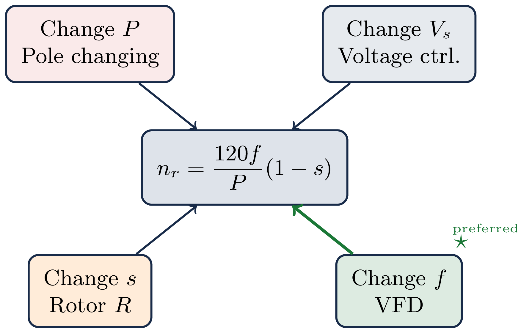
Speed Control — The Fundamental Equation

Three Independent Handles for Speed Control

n_r = n_s(1−s) = (120f/P)(1−s)

Table 3 — Speed Control Methods Summary
Change	Method	Quality
Poles P	Pole changing	Steps only
Voltage V_s	Thyristor control	Limited range; poor efficiency
Slip s	Rotor resistance	Wide range; very poor efficiency
Frequency f	VFD (V/f control)	Excellent

🎯

Efficiency Is the Discriminator

VFD changes n_s directly — slip remains small at all speeds

All methods except frequency control waste power in external resistors or operate at high slip where P_r,Cu = s·P_ag is large. With VFD, s ≈ 3–5% at all operating speeds, giving consistently high efficiency.

Overview block diagram of speed control methods for polyphase induction motors: pole changing, voltage control, rotor resistance, and VFD — Fig. 6 — Speed control overview: three handles are poles P, voltage V_s, and frequency f.

SECTION 09

Method 1 — Pole Changing

A specially wound stator is reconnected to change the number of poles, shifting the synchronous speed in discrete steps using consequent-pole winding.

Table 4 — Common Speed Pairs at 50 Hz
Pole Configuration P₁/P₂	Speed 1 (rpm)	Speed 2 (rpm)
4 / 8	1500	750
4 / 6	1500	1000
6 / 8	1000	750

When to Use

2–3 fixed speeds are sufficient (e.g. multi-speed fans, escalators)
Simple control — no power electronics
Examples: cooling tower fans, machine-tool spindles

Limitations

Only discrete speed steps — no continuous variation
Special motor required (2 speeds: 1 winding; 3 speeds: 2 windings)
Motor is physically larger than a single-speed equivalent

SECTION 10

Method 2 — Voltage Control

Thyristor AC voltage controllers reduce V_s. Since T_em ∝ V_s², the torque-speed curve shifts downward — the motor settles at higher slip to match the load torque, resulting in lower speed.

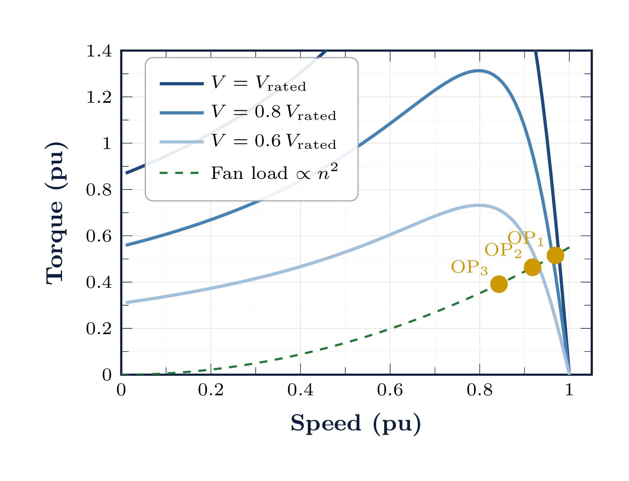
Family of torque-speed curves under reduced stator voltage showing the operating point shift to higher slip — Fig. 7 — Voltage control: reduced V_s shifts T-n curve down; efficiency poor at high slip.

Why Not for Constant-Torque Loads?

The operating point slides deep into the high-slip region. At 50% speed: s ≈ 0.5 and P_r,Cu = s·P_ag = 0.5·P_ag. Half of all converted power is wasted as rotor heat. The rotor overheats and efficiency collapses.

Useful range for fan/pump loads (T_L ∝ n²): approximately 70–100% of rated speed only.

SECTION 11

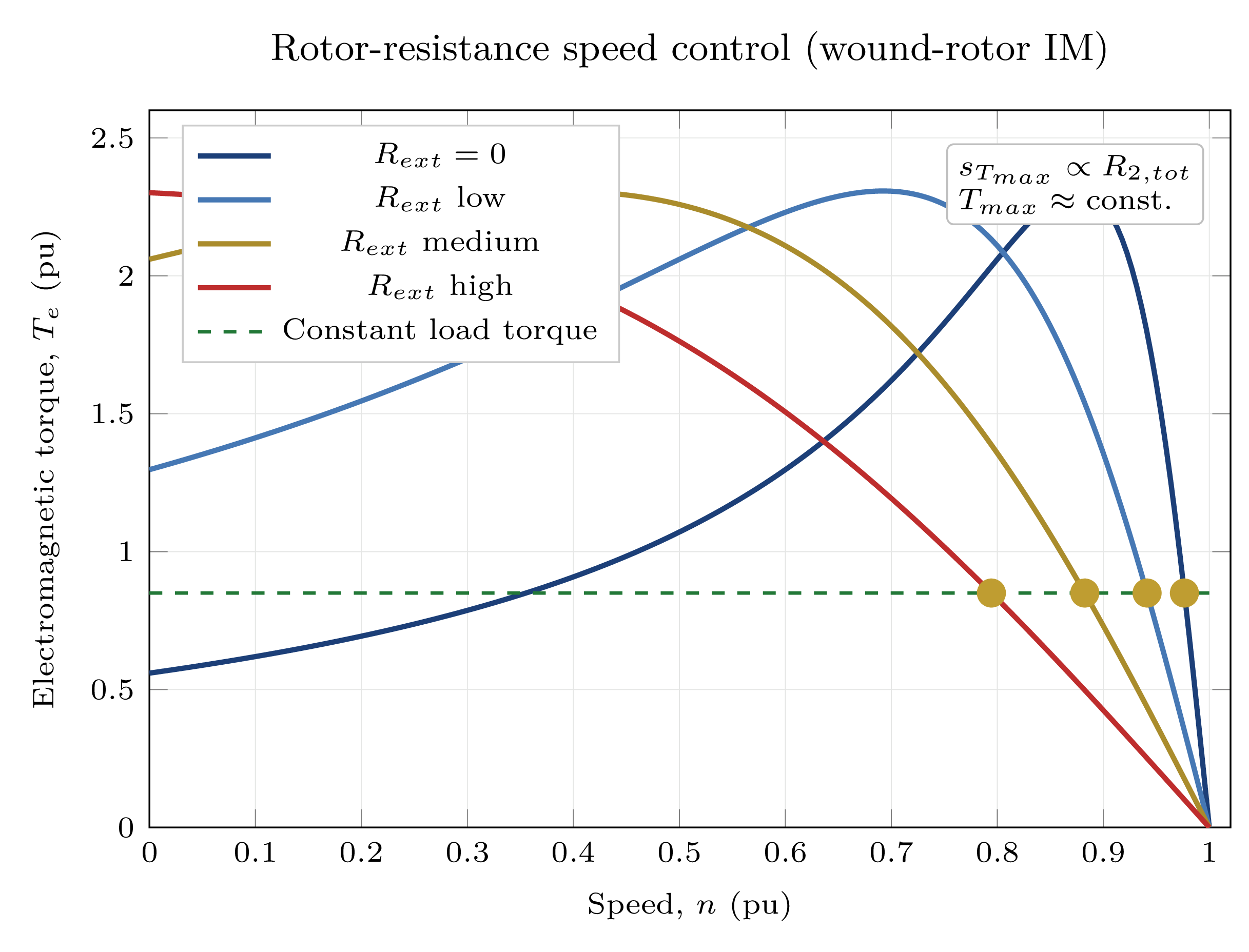
Method 3 — Rotor Resistance Speed Control

Operating Point with External Resistance

s_op ≈ [(R_r′ + R_ext) / R_r′] · s_rated

Mechanical efficiency: η_mech ≈ 1 − s

Modern Status — Almost Entirely Replaced by VFDs

At 50% speed (s = 0.5): only 50% of air-gap power reaches the shaft. P_loss,ext = 3·R_ext·I_r′². The severe efficiency penalty at reduced speeds makes this approach economically unacceptable for new installations.

Rotor resistance speed control torque-speed characteristics showing operating points at different external resistance values — Fig. 8 — Rotor resistance speed control: operating point slides to higher slip; η_mech ≈ 1−s.

SECTION 12

Variable Frequency Drive — Architecture & Power Stages

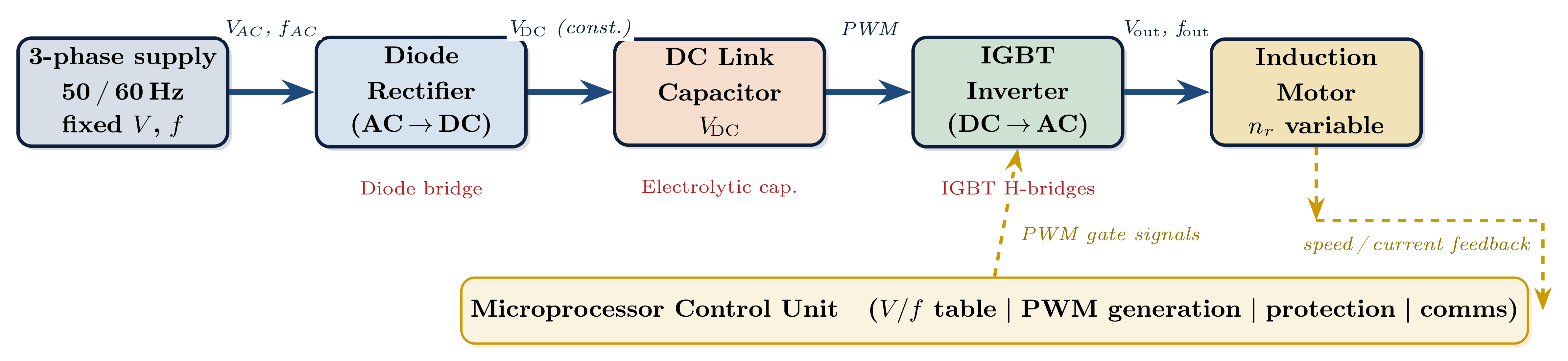
Fig. 2 — Three-stage VFD: diode rectifier (AC→DC), DC link capacitor bank, IGBT PWM inverter (DC→variable AC).

⚡PWM Inverter

IGBTs switch at 4–16 kHz. The motor's inductance filters the pulses to produce approximately sinusoidal fundamental currents at the desired output frequency f_out.

Smooth Starting Capability

VFD ramps from f ≈ 0 Hz. Slip stays small; current remains near rated value throughout. No inrush current and no voltage dip on the supply.

SECTION 13

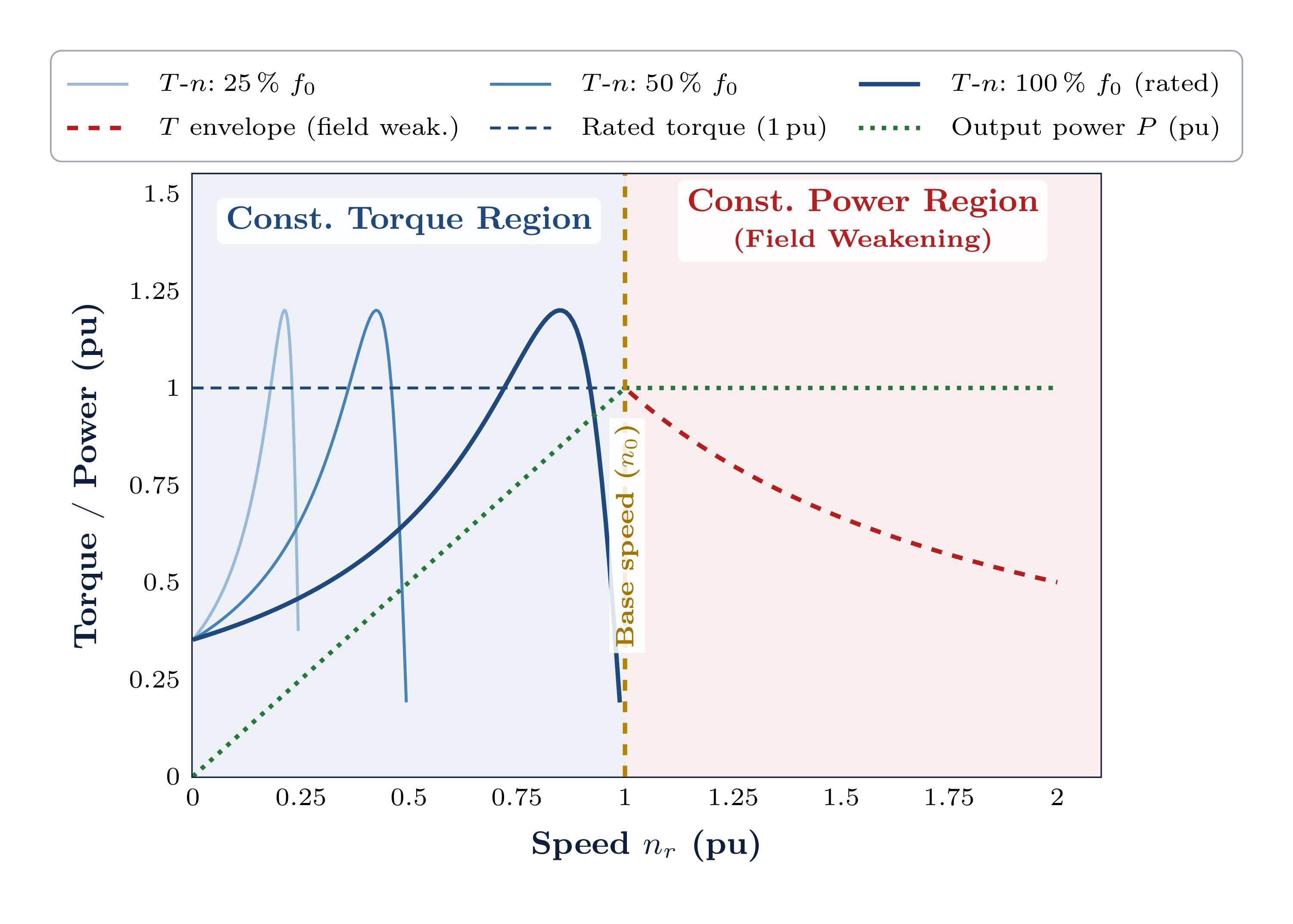
V/f Control — Constant Flux Principle

The stator voltage equation (neglecting R_s drop at normal speed):

Constant Flux Derivation

V_s ≈ E_ag = 4.44·f·N_s·Φ_max

∴ Φ_max = V_s / (4.44·f·N_s) ∝ V/f

If V/f = const ⟹ Φ_max = const
Constant flux ⟹ constant torque capability at every speed

⬇️Below Base Speed (f < f_rated)

V/f = const ⇒ Φ = const
T_max approximately constant
Small slip ⇒ high efficiency
Constant-torque region

⬆️ Above Base Speed (f > f_rated)

Voltage saturates at V_max
Flux decreases as f rises
T_max ∝ 1/f — torque capability falls
Output power remains approximately constant
Field-weakening region

Low-Speed Voltage Boost

At low f, stator resistance drop I_sR_s is not negligible. A boost is added:

V_boost(f) = V_min + [(V_rated−V_min)/f_rated] · f

V_min ≈ 15–25% of V_rated

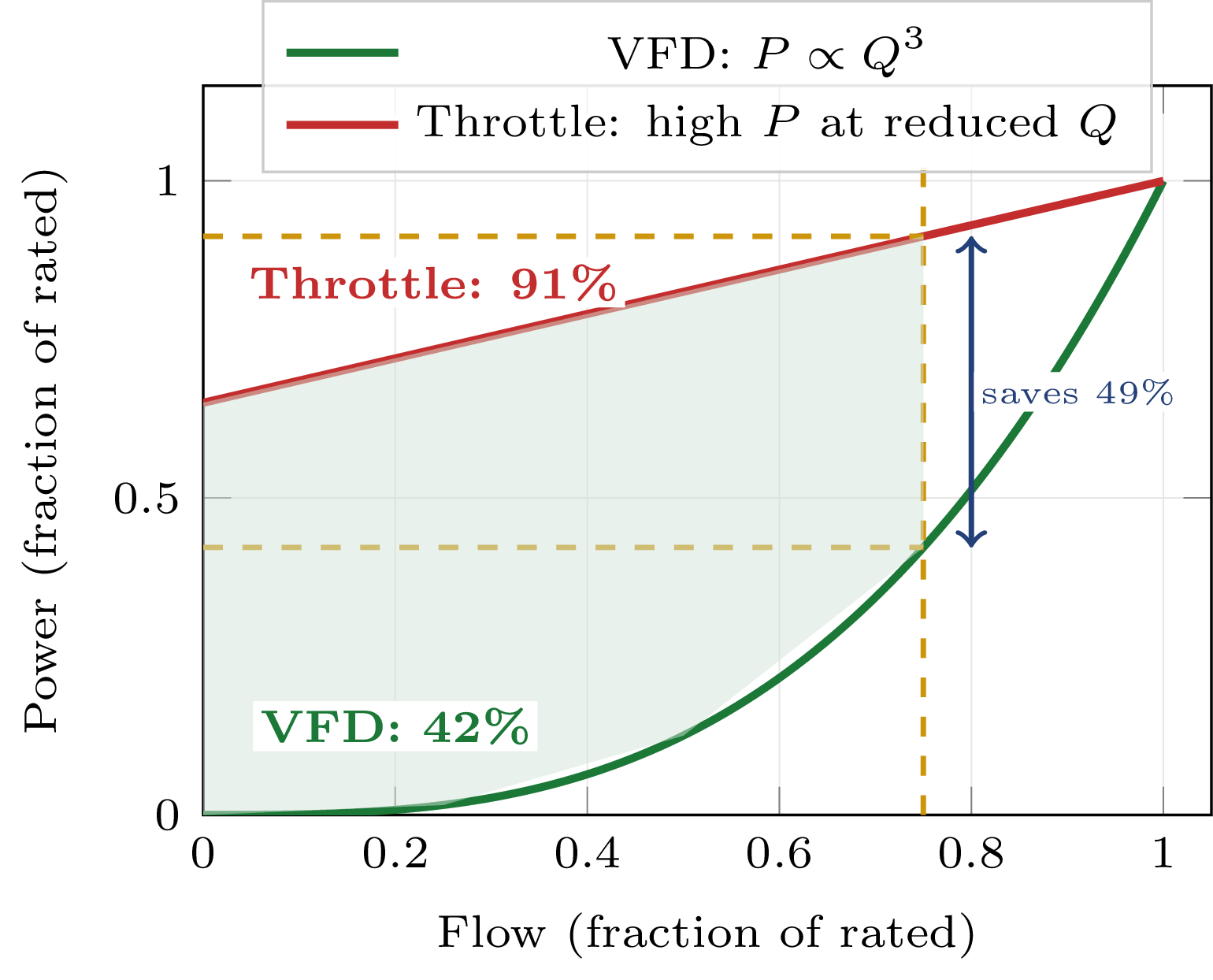
VFD torque-speed characteristics showing the constant-torque region below base speed and the field-weakening region above — Fig. 11 — VFD regions: constant-torque (V/f=const, below f_rated) and field-weakening (above f_rated).

SECTION 14

Affinity Laws & VFD Energy Savings

The Affinity Laws — Centrifugal Fans, Pumps & Compressors

Q₂/Q₁ = n₂/n₁ (Flow ∝ speed)
H₂/H₁ = (n₂/n₁)² (Head ∝ speed²)
P₂/P₁ = (n₂/n₁)³ (Power ∝ speed³)

💰

The Cube Law — Critical Insight

Reducing speed to 75% cuts power to just 42% of full-speed demand

0.75³ = 0.422. This cube relationship makes even modest speed reductions yield enormous energy savings — and explains why VFDs are among the most cost-effective investments in industrial energy management.

Throttle Valve at 75% Flow

Motor runs at full speed; valve dissipates excess energy. Power ≈ 75–100% of rated. All energy above the process requirement is wasted as pressure drop across the valve.

VFD at 75% Flow

Motor runs at 75% speed. Power ≈ 42% of rated. No throttling loss. Energy saving ≈ 33–58%. Payback period typically 1–3 years.

Energy comparison chart between throttle valve control and VFD speed control at various flow rates showing VFD energy savings — Fig. 12 — VFD vs. throttle valve: at 75% flow, VFD uses ~42% of full-speed power vs. ~80–100% for throttling.

SECTION 15

Lecture Summary

Starting Methods

Method	I_st/I_r	T_st/T_DOL
DOL	5–7×	100%
Y-Δ	1.7–2.3×	33%
Autotransformer	2–3×	Selectable
Soft starter	2–4×	Variable
VFD	<1.5×	>150%

Speed Control Methods

Method	Range	Efficiency
Pole changing	Discrete steps	Good
Voltage control	70–100%	Poor
Rotor resistance	0–100%	Very poor
VFD (V/f)	0–>100%	Excellent

V/f Control Principle

V_s/f = const ⇒ Φ = const ⇒ Constant torque capability
Below base speed: constant-torque region
Above base speed: field-weakening (constant power)
Slip small at all speeds ⇒ high efficiency everywhere

Affinity Laws

P ∝ n³ ⇒ P₂/P₁ = (n₂/n₁)³

Reducing speed to 75% → power drops to 42%
Energy savings of 30–60% for fans/pumps
VFD payback: typically 1–3 years

🏆The Modern Conclusion

The Variable Frequency Drive (VFD) is the universal solution for induction motor drives. It solves the starting problem, enables continuous speed control with high efficiency, maintains small slip at all operating points, leverages the cube law for centrifugal loads, and typically pays back its cost in energy savings within 1–3 years. For new industrial installations, the VFD is the first choice — not the last resort.