Lecture 5B: Equivalent Circuit & Power Flow | Polyphase Induction Machines

RECAP

Key Results from Lecture 5A

✓Established Results

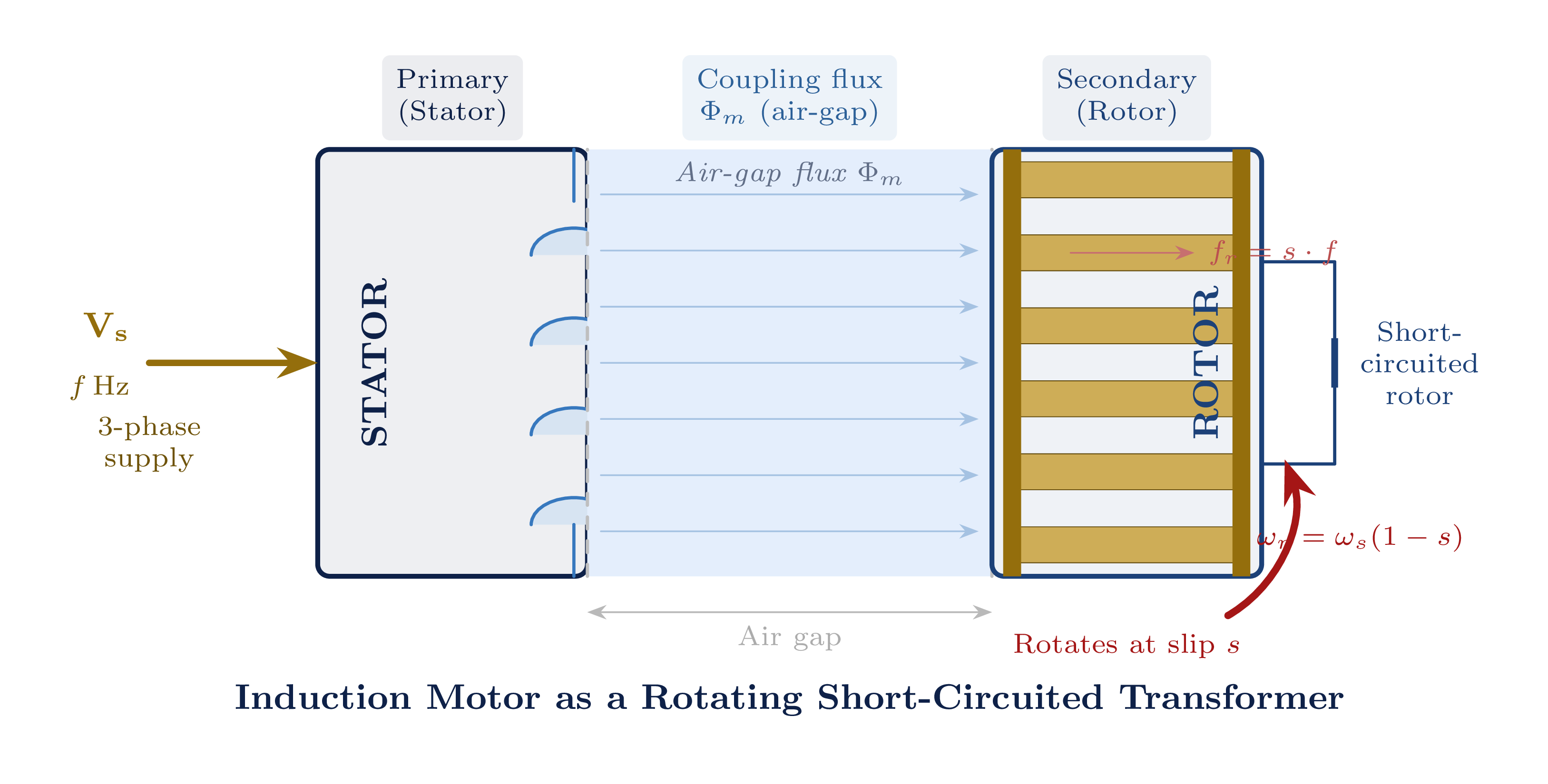
Rotating field at synchronous speed: \(n_s = \dfrac{120f}{P}\) rpm
Slip: \(s = \dfrac{n_s - n_r}{n_s}\), rotor frequency \(f_r = s \cdot f\)
Rotor speed: \(\omega_r = \omega_s(1-s)\)
Rotor must slip to sustain torque
Typical rated slip: 0.5%–8%

Today's Objectives

Transformer analogy & turns-ratio referral
Per-phase equivalent circuit (full & simplified)
Physical meaning of every circuit element
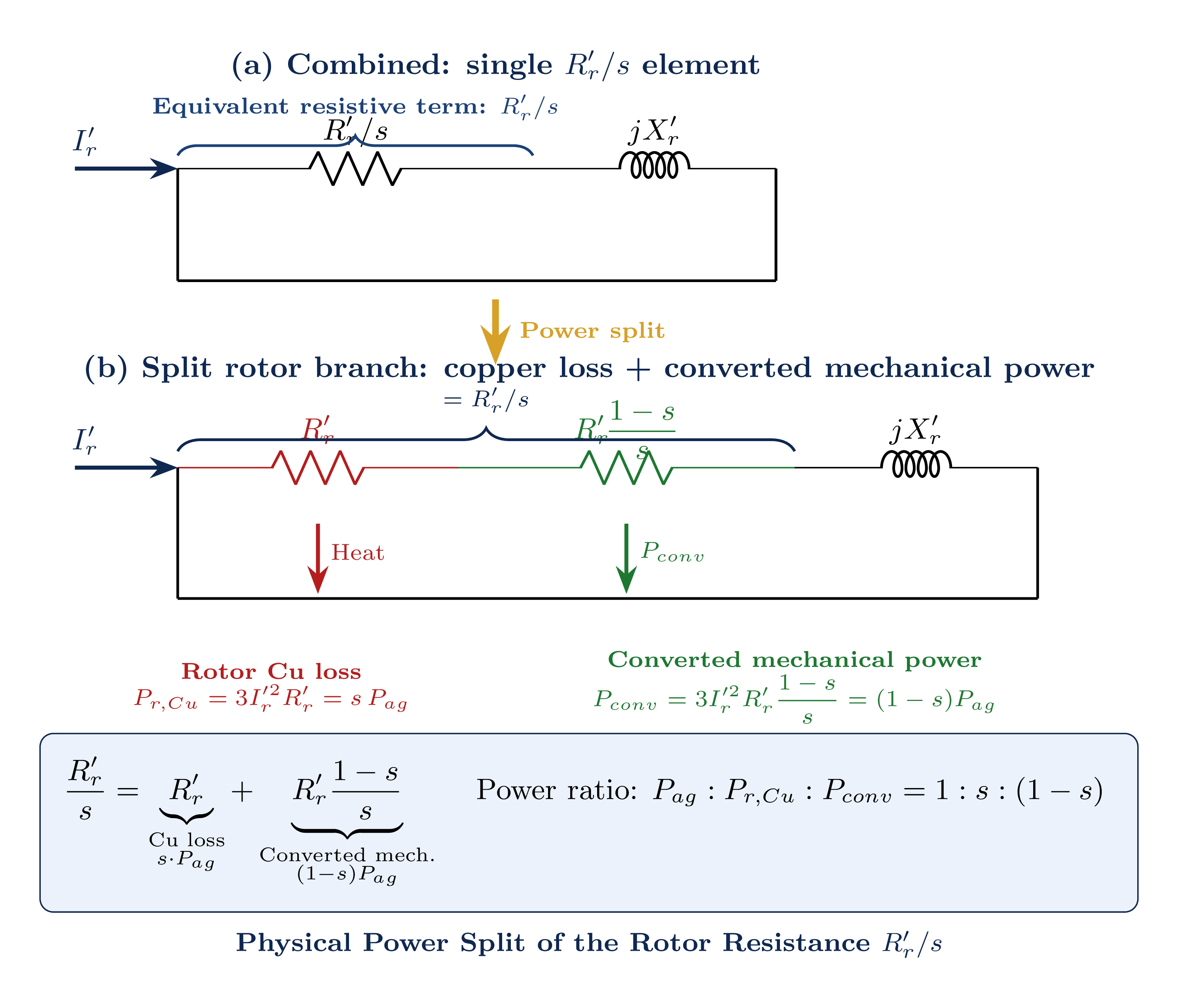
The critical \(R_r'/s\) power split
Complete power flow analysis & torque expression
Efficiency & power factor vs. load

SECTION 01

Why Do We Need an Equivalent Circuit?

🎯Objectives

Predict torque, current, PF, efficiency at any operating point — no prototype needed
Provide the mathematical basis for drive control design
Enable parameter extraction from standard motor tests (Lecture 5C)

What the Model Gives Us

Quantity	From Circuit
Stator current \(I_s\)	KVL
Rotor current \(I_r'\)	KVL
Input power \(P_{in}\)	\(3V_s I_s \cos\phi\)
Air-gap power \(P_{ag}\)	\(3I_r'^{\,2} R_r'/s\)
Torque \(T_{em}\)	\(P_{ag}/\omega_s\)
Efficiency \(\eta\)	\(P_{out}/P_{in}\)

📋 Scope: The per-phase steady-state equivalent circuit assumes balanced 3-phase supply, symmetrical machine, constant rotor speed, and sinusoidal air-gap flux distribution.

SECTION 02

The Transformer Analogy

Table 1 — Transformer vs. Induction Motor
Transformer	Induction Motor
Primary winding	Stator winding
Secondary winding	Rotor winding
Magnetic core	Air-gap flux path
Open/loaded secondary	Short-circuited rotor
Fixed secondary	Rotating secondary
Fixed frequency	Slip frequency \(f_r = sf\)

⚡

The Crucial Difference

The rotating secondary introduces a slip-dependent rotor impedance

This feature — the slip-dependent impedance \(R_r'/s\) — separates induction motor analysis from ordinary transformer analysis and is the key to understanding all operating characteristics.

Transformer analogy diagram showing stator as primary and rotor as rotating secondary winding — Transformer analogy: stator (primary) vs. rotor (rotating short-circuited secondary).

SECTION 03

Turns-Ratio Referral — Rotor to Stator

Stator and rotor have different numbers of turns. To place them in one circuit, rotor quantities are scaled to the stator side using the effective turns ratio:

Turns Ratio & Referral Equations

\[a = \frac{N_s}{N_r}\] \[R_r' = a^2 R_r \qquad \text{(referred rotor resistance)}\] \[L_r' = a^2 L_r \qquad \text{(referred rotor leakage inductance)}\] \[X_r' = a^2 X_r \qquad \text{(referred rotor leakage reactance)}\] \[I_r' = \frac{I_r}{a} \qquad \text{(referred rotor current)}\] \[E_r' = a\,E_r \qquad \text{(referred rotor voltage)}\]

🔑 Prime (′) Notation: All rotor quantities in the equivalent circuit (\(R_r'\), \(X_r'\), \(I_r'\)) are referred to the stator side. After referral: \(E_{ag} = E_r'\), allowing physical isolation between stator and rotor circuits to be removed.

SECTION 04

Slip-Dependent Rotor Impedance

At rotor frequency \(f_r = sf\), the per-phase rotor voltage equation is:

Rotor Circuit at Slip Frequency → Referred Impedance

\[s\,E_{ag} = I_r\bigl(R_r + j\,s\,X_r\bigr)\]

Dividing by \(s\):

\[E_{ag} = I_r\!\left(\frac{R_r}{s} + jX_r\right)\]

After referral:

\[\boxed{E_{ag} = I_r'\!\left(\frac{R_r'}{s} + jX_r'\right)}\]

Table 2 — Impedance vs. Slip
Slip \(s\)	\(R_r'/s\)	Behaviour
\(s = 1\) (standstill)	\(R_r'\)	High current
\(s = 0.05\) (rated)	\(20R_r'\)	Moderate current
\(s \to 0\) (synchronous)	\(\to \infty\)	No current, no torque

💡 Key Insight: \(X_r'\) is evaluated at stator frequency \(f\). Slip appears only in the resistance term \(R_r'/s\). As the motor accelerates (slip ↓), \(R_r'/s\) ↑ — rotor current naturally decreases even at constant supply voltage.

SECTION 05

Full Per-Phase Equivalent Circuit

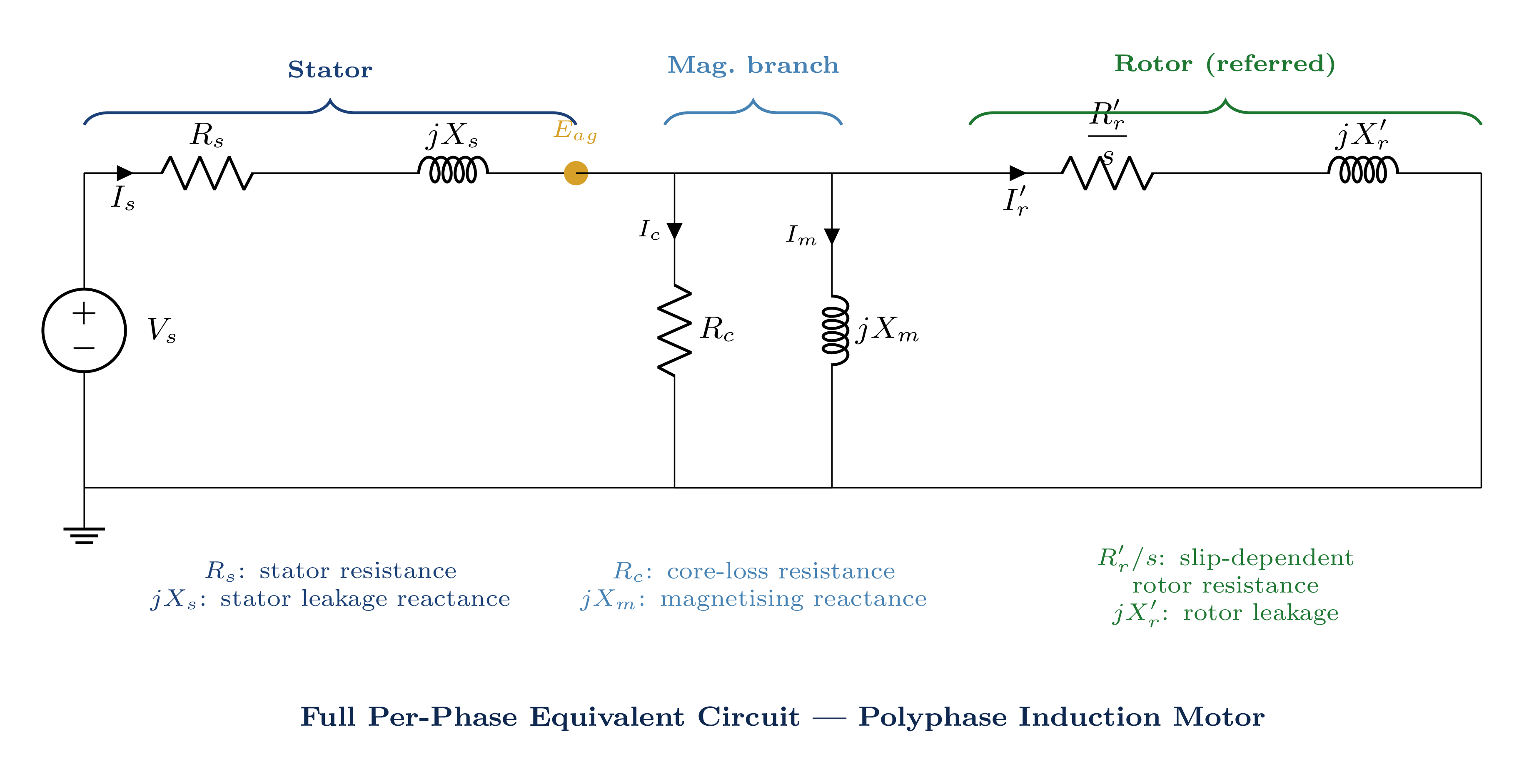
Fig. 1 — Full per-phase equivalent circuit: stator (\(R_s\), \(jX_s\)), magnetising branch (\(R_c \parallel jX_m\)), rotor (\(R_r'/s\), \(jX_r'\)).

SECTION 06

Physical Meaning of Circuit Elements

Table 3 — Circuit Element Reference
Region	Symbol	Name	Physical Meaning
Stator	\(R_s\)	Stator resistance	Copper losses in stator windings: \(P_{s,Cu} = 3I_s^2 R_s\)
Stator	\(jX_s\)	Stator leakage reactance	Flux linking only the stator; \(X_s = \omega_e L_{ls}\)
Magnetising	\(R_c\)	Core-loss resistance	Iron losses (hysteresis + eddy current); \(P_{core} = 3E_{ag}^2/R_c\)
Magnetising	\(jX_m\)	Magnetising reactance	Main mutual flux; \(I_m \approx 25\text{–}40\%\, I_{rated}\)
Rotor	\(R_r'/s\)	Referred rotor resistance	Key element — contains both rotor Cu loss and mechanical output power
Rotor	\(jX_r'\)	Referred rotor leakage	Flux linking only rotor; \(X_r' = \omega_e L_{lr}'\); evaluated at stator frequency

📌 Note on \(R_c\): \(R_c\) is very large and absorbs negligible current. It is often neglected (lumped into no-load losses) or treated as a constant fixed loss. The simplified circuit retains only \(jX_m\).

SECTION 07

The Critical Power Split of \(R_r'/s\)

Resistance Split: Copper Loss + Mechanical Output

\[\boxed{\frac{R_r'}{s} = \underbrace{R_r'}_{\text{Rotor Cu loss}} + \underbrace{R_r'\,\dfrac{1-s}{s}}_{\text{Mechanical output}}}\]

🔥\(R_r'\) — Real Resistor

Heat dissipated in rotor bars. This is an actual physical resistor and represents true copper loss.

Rotor Copper Loss

\[P_{r,Cu} = 3I_r'^{\,2}\,R_r' = s\cdot P_{ag}\]

⚙️\(R_r'(1-s)/s\) — Fictitious Resistor

Circuit representation of shaft work. Not a physical component — it is the circuit proxy for mechanical work done on the load.

Mechanical Output

\[P_{conv} = 3I_r'^{\,2}\,R_r'\,\frac{1-s}{s} = (1-s)\,P_{ag}\]

SECTION 08

Simplified Per-Phase Equivalent Circuit

In most calculations \(R_c\) is very large and absorbs negligible current. The magnetising branch reduces to a single shunt element \(jX_m\).

KCL at the Air-Gap Node

\[\vec{I}_s = \vec{I}_m + \vec{I}_r'\]

Simplified per-phase equivalent circuit of the induction motor with core-loss resistance R_c neglected — Fig. 3 — Simplified equivalent circuit (\(R_c\) neglected); most commonly used in practice.

Typical Current Magnitudes

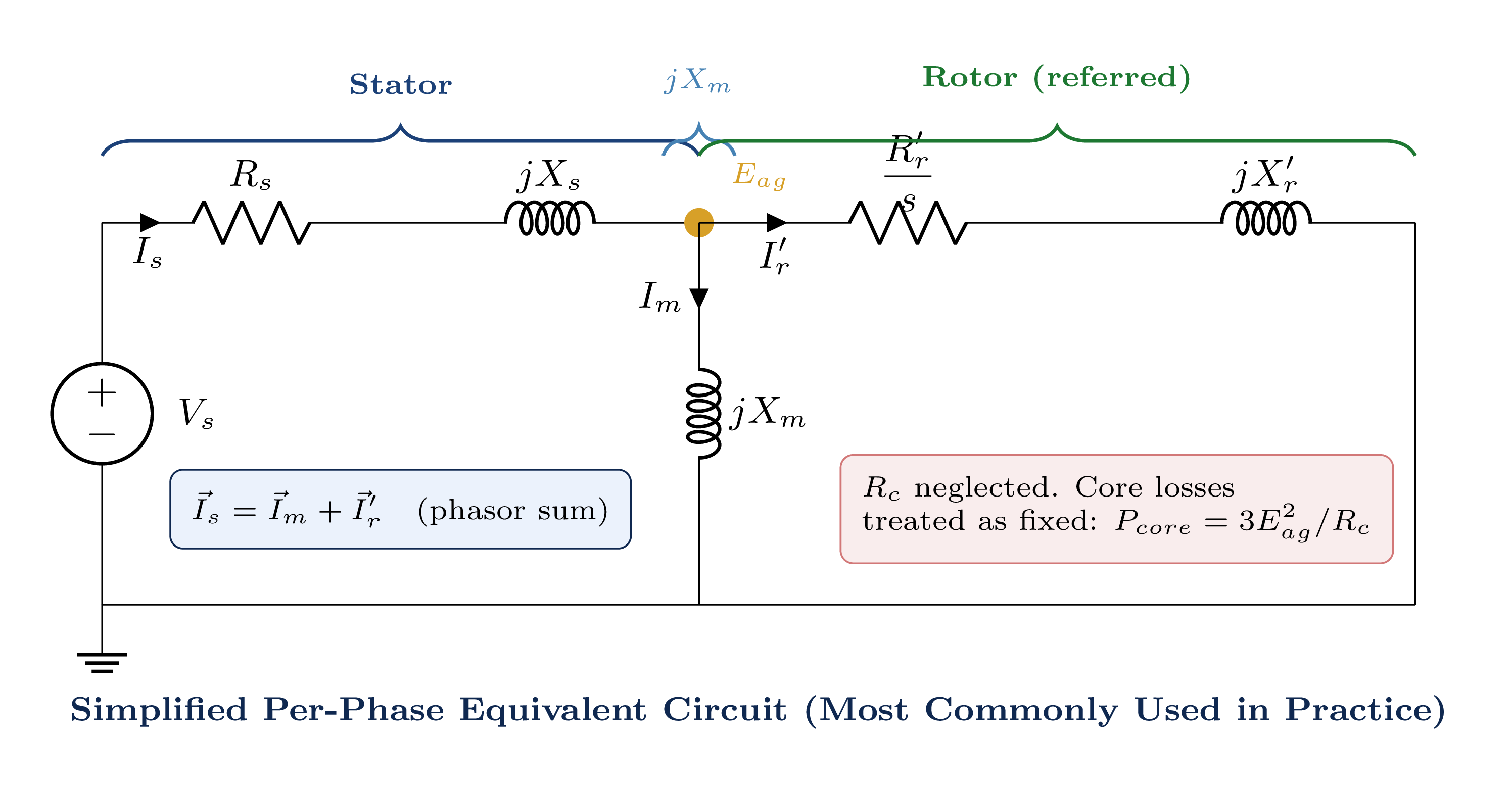
\(I_m \approx 25\text{–}40\%\) of \(I_{rated}\)
\(I_r' \approx 90\text{–}100\%\) of \(I_{rated}\) at full load

SECTION 09

Phasor Diagram

📐Step-by-Step Construction

Take \(E_{ag}\) as the reference phasor
\(I_m\) lags \(E_{ag}\) by \(90°\) (purely inductive \(jX_m\))
\(I_r'\) lags \(E_{ag}\) by \(\theta_r = \arctan(sX_r'/R_r')\) — small at rated slip
\(\vec{I}_s = \vec{I}_m + \vec{I}_r'\) (phasor sum)
\(\vec{V}_s = \vec{E}_{ag} + \vec{I}_s(R_s + jX_s)\)

\(\phi\) = angle between \(V_s\) and \(I_s\) = power factor angle

Phasor diagram of the induction motor showing stator voltage, rotor current, magnetising current, and power factor angle — Fig. 4 — Phasor diagram at rated load: \(V_s\), \(I_s\), \(I_m\), \(I_r'\) and power factor angle \(\phi\).

Why Power Factor is Always Lagging

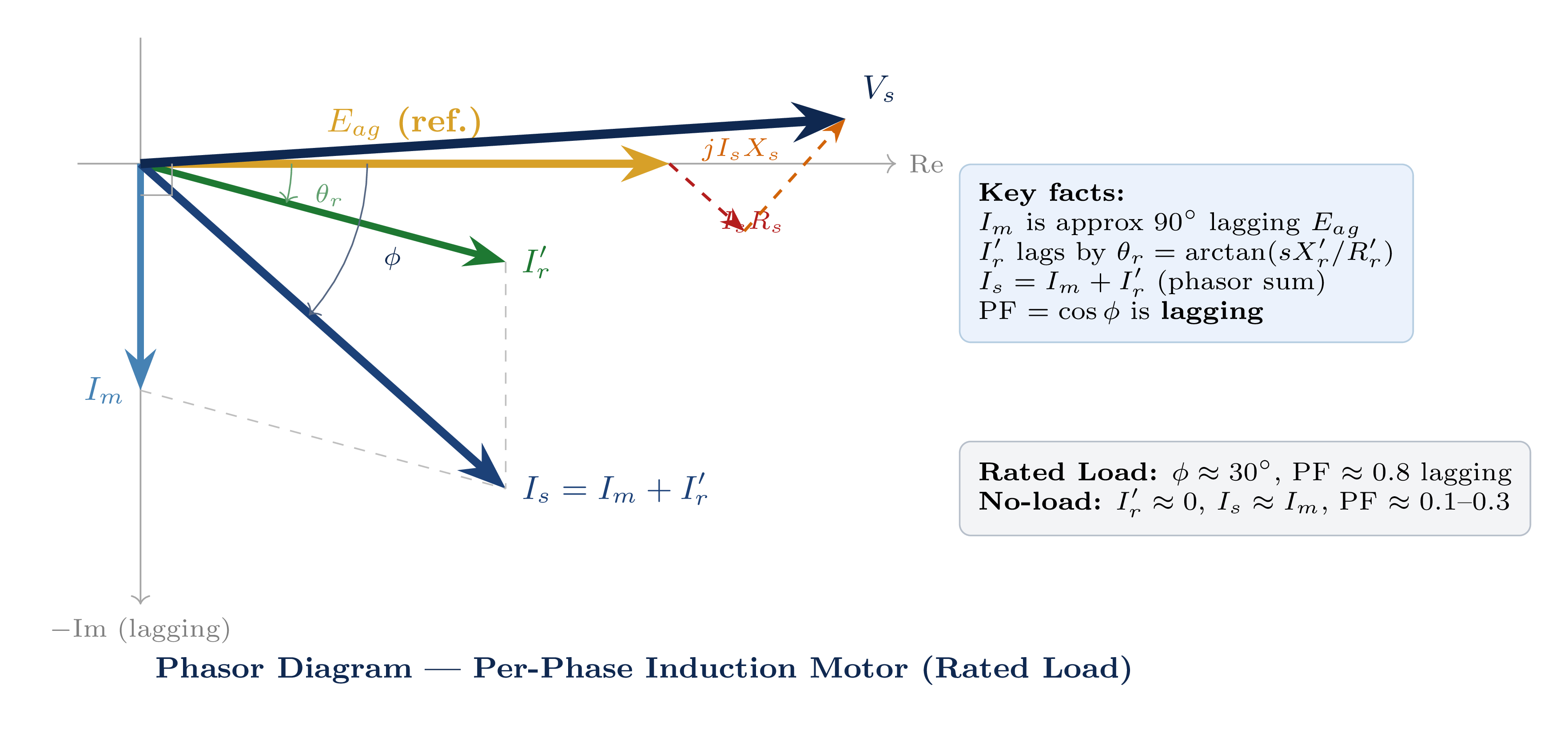
\(I_m\) is always \(90°\) lagging regardless of load. Even at full load, \(I_s\) carries a substantial reactive component — the "magnetising current penalty."

Condition	PF Angle \(\phi\)	Power Factor	Notes
No-load	80°–85°	0.1–0.3	\(I_s \approx I_m\); purely reactive
Rated load	25°–40°	0.75–0.90	\(I_r'\) significant; \(I_m\) still present

SECTION 10

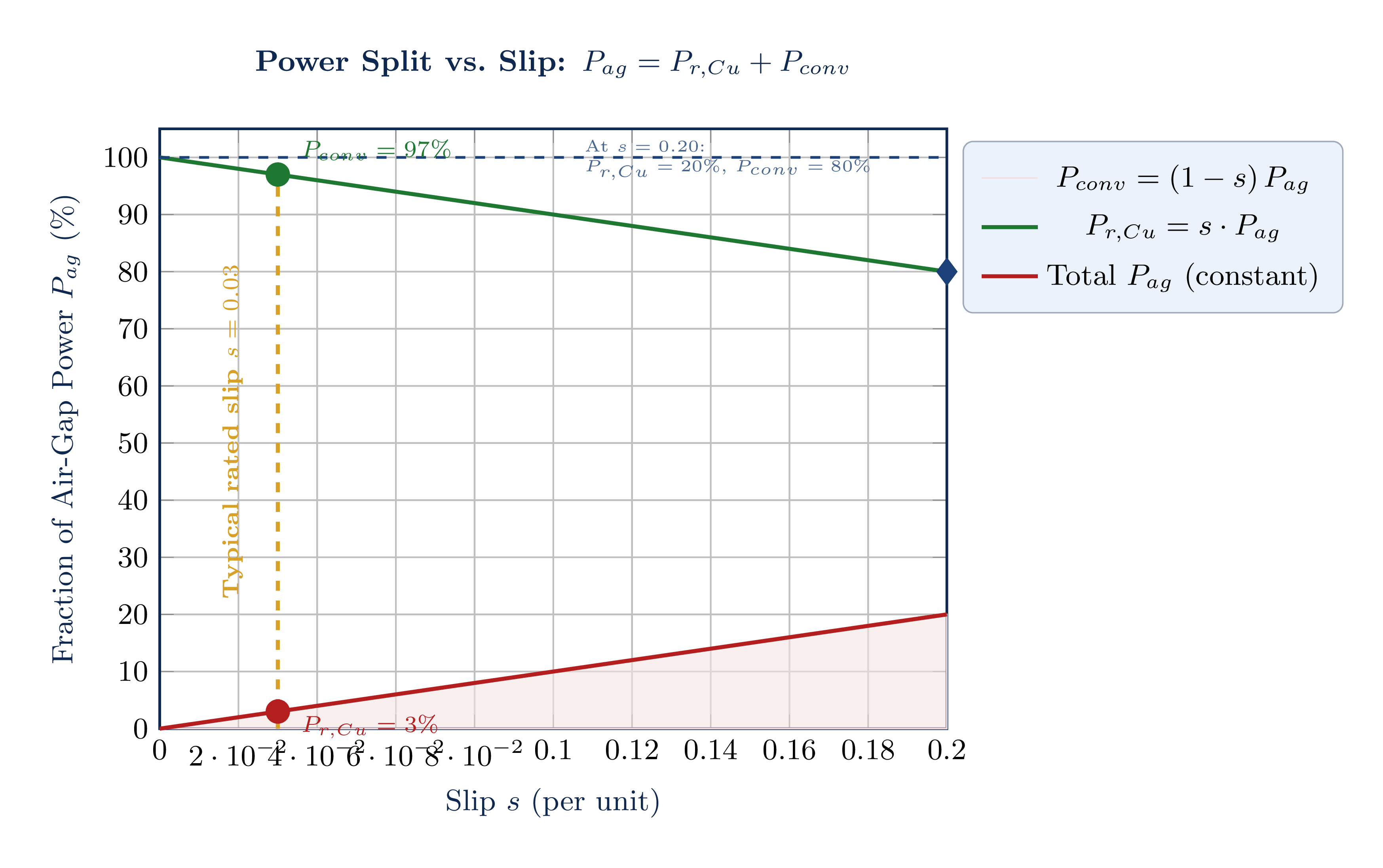
Power Flow Analysis — The Complete Chain

Power flow chain diagram from three-phase electrical input through stator, air gap, and rotor to mechanical shaft output — Fig. 5 — Power flow chain: \(P_{in} \to P_{ag} \to P_{conv} \to P_{out}\).

PInput Power (3-phase)

\[P_{in} = 3\,V_s\,I_s\cos\phi\]

CStator Copper Loss

\[P_{s,Cu} = 3\,I_s^2\,R_s\]

AAir-Gap Power

\[P_{ag} = P_{in} - P_{s,Cu} - P_{core} = 3\,I_r'^{\,2}\,\frac{R_r'}{s}\]

RRotor Copper Loss

\[P_{r,Cu} = 3\,I_r'^{\,2}\,R_r' = s\cdot P_{ag}\]

MConverted Power

\[P_{conv} = (1-s)\,P_{ag}\]

OShaft Output Power

\[P_{out} = P_{conv} - P_{fw}\]

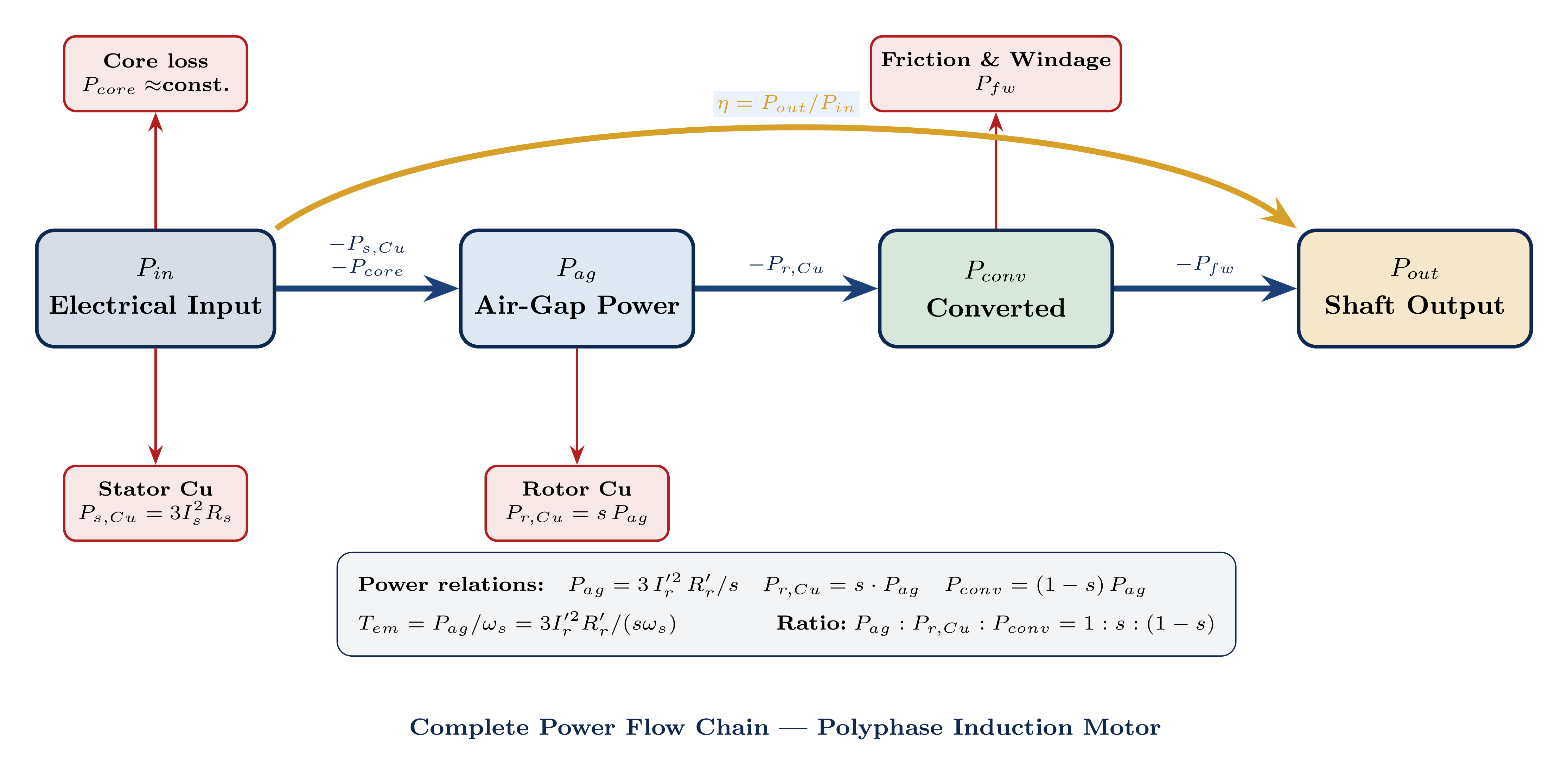
\(P_{fw}\) = friction & windage losses

⚖️

Fundamental Power Ratio

\[P_{ag} : P_{r,Cu} : P_{conv} = 1 : s : (1-s)\]

At \(s = 0.03\): only 3% of air-gap power is lost as rotor heat. Large motors use very small rated slip (0.5–2%) to achieve high efficiency — at \(s = 0.01\), only 1% of air-gap power is wasted.

Graph of air-gap power, rotor copper loss, and converted power fractions versus slip for an induction motor — Fig. 6 — Power ratio vs. slip: \(P_{r,Cu}/P_{ag} = s\) and \(P_{conv}/P_{ag} = 1-s\).

SECTION 11

Electromagnetic Torque

Torque–Power Linkage

\[P_{conv} = T_{em}\,\omega_r = T_{em}\,\omega_s(1-s)\] \[P_{ag} = T_{em}\,\omega_s\] \[\boxed{T_{em} = \frac{P_{ag}}{\omega_s} = \frac{3\,I_r'^{\,2}\,R_r'}{s\,\omega_s}}\]

Table 4 — Three Equivalent Forms of Torque
Approach	Formula
From \(P_{ag}\)	\(T_{em} = \dfrac{P_{ag}}{\omega_s}\)
From \(P_{conv}\)	\(T_{em} = \dfrac{P_{conv}}{\omega_r}\)
From circuit	\(T_{em} = \dfrac{3\,I_r'^{\,2}\,R_r'}{s\,\omega_s}\)

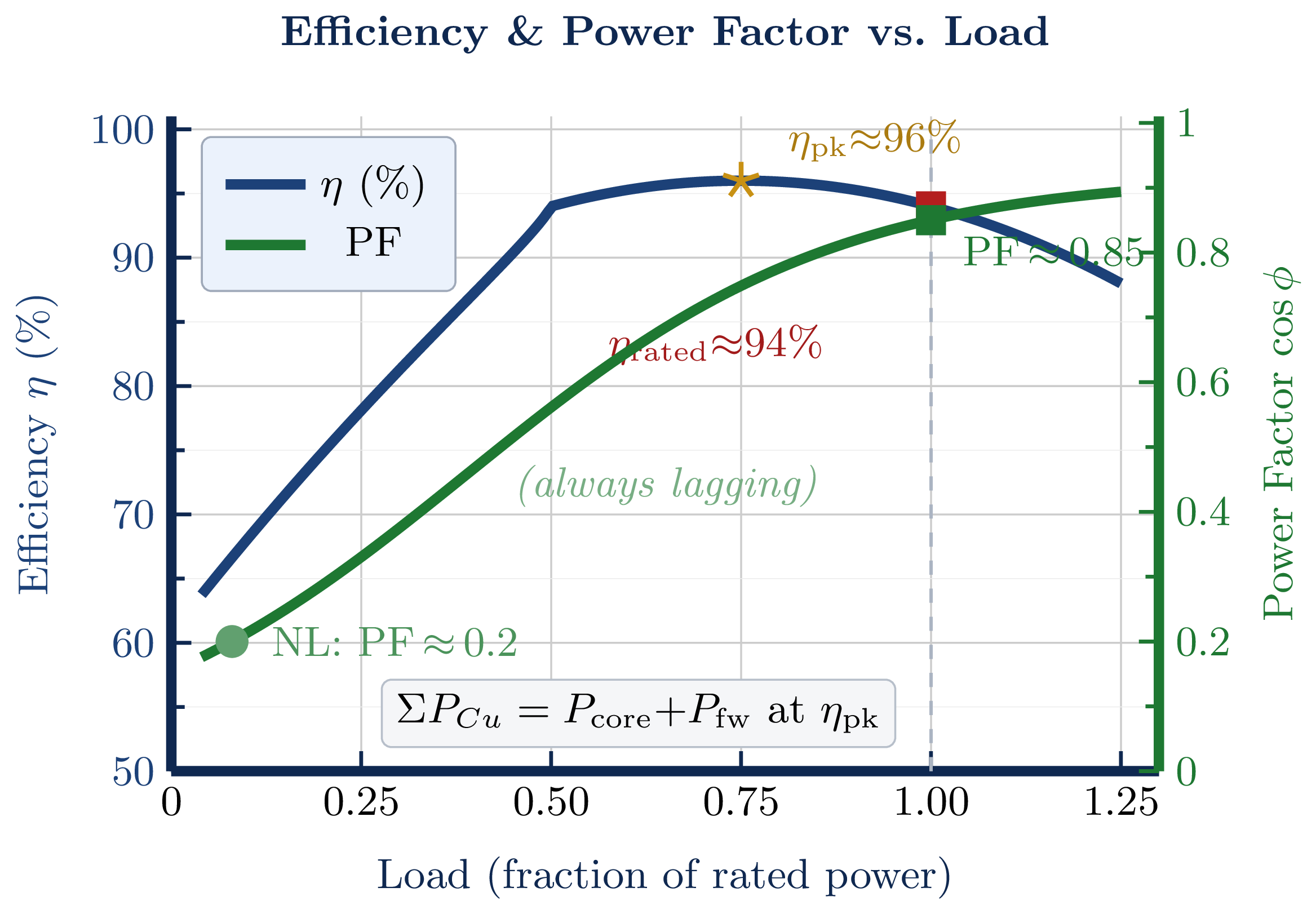
📌 Torque is set by air-gap power and synchronous (not rotor) speed. At constant \(V_s\) and \(\omega_s\), torque is controlled via slip (which controls \(I_r'\)). This is the foundation for the torque-slip equation in Lecture 5C.

SECTION 12

Efficiency & Power Factor vs. Load

ηEfficiency

\[\eta = \frac{P_{out}}{P_{in}} = \frac{P_{in} - \Sigma P_{loss}}{P_{in}}\]

Variable losses: \(P_{s,Cu}\), \(P_{r,Cu}\) (rise with load)
Fixed losses: \(P_{core}\), \(P_{fw}\) (approx. constant)

φPower Factor

\[\mathrm{PF} = \cos\phi = \frac{P_{in}}{3\,V_s\,I_s}\]

Always lagging due to \(I_m\) component. Poor at light loads.

Table 5 — Typical Values at Rated Load
Motor Size	Efficiency \(\eta\)	Power Factor
Small (<5 kW)	75–88%	0.70–0.80
Medium (5–100 kW)	88–94%	0.80–0.87
Large (>100 kW)	93–97%	0.85–0.92

At Light Loads — Both \(\eta\) and PF Degrade Significantly

Fixed losses dominate \(P_{in}\)
\(I_s \approx I_m\) ⇒ very low PF
Running oversized motors at light load wastes energy
Peak efficiency occurs at approximately 75% rated load where variable losses equal fixed losses

Graph of efficiency and power factor versus per-unit load for a typical polyphase induction motor — Fig. 7 — Efficiency \(\eta\) and power factor \(\cos\phi\) vs. load; peak \(\eta \approx 75\%\) rated load.

SECTION 13

Lecture Summary

1. Transformer Analogy

Stator = primary; Rotor = short-circuited rotating secondary
Referred quantities: \(R_r' = a^2 R_r\), \(X_r' = a^2 X_r\), \(a = N_s/N_r\)

2. Equivalent Circuit

Full: \(R_s\), \(jX_s\), \(R_c \parallel jX_m\), \(R_r'/s\), \(jX_r'\)
Simplified: drop \(R_c\); use \(jX_m\) shunt only

3. Power Split of \(R_r'/s\)

\[\frac{R_r'}{s} = R_r' + R_r'\,\frac{1-s}{s} \quad \text{(Cu loss + mechanical output)}\]

4. Power Flow

\(P_{ag} : P_{r,Cu} : P_{conv} = 1 : s : (1-s)\)
\(T_{em} = \dfrac{P_{ag}}{\omega_s} = \dfrac{3\,I_r'^{\,2}\,R_r'}{s\,\omega_s}\)

5. Phasor Diagram

\(I_m\) always \(90°\) lagging ⇒ PF always lagging
No-load: \(I_s \approx I_m\), very low PF
Rated load: PF ≈ 0.75–0.90

Next: Lecture 5C

Torque-slip characteristics via Thévenin equivalent, maximum torque analysis, NEMA design classes, and parameter measurement from standard motor tests.