- Identify the amplitude, angular frequency, period, frequency and phase of a sinusoid.
- Determine whether one sinusoid leads or lags another, converting sines to cosines first.
- Work fluently with complex numbers in rectangular, polar and exponential form.
- Transform between the time domain and the phasor domain in both directions.
- State the phasor \(v\)–\(i\) relationship for a resistor, inductor and capacitor.
- Compute impedance and admittance, and separate them into resistance/reactance and conductance/susceptance.
- Apply KVL, KCL, series–parallel reduction and the divider rules to phasor circuits.
- Find the input impedance of a network at a stated frequency.
- Explain how an RC network produces a controlled phase shift, and how an AC bridge measures an unknown impedance.
Introduction
Part 1 is complete, and with it the treatment of DC circuits and their transients. From here the sources are sinusoidal, and the question changes: instead of asking what happens in the moments after a switch operates, we ask what the circuit settles down to and stays doing indefinitely — the sinusoidal steady state.
Why sinusoids in particular? Three reasons, and each is sufficient on its own. Rotating machinery naturally generates them, so the entire electrical supply of the world is sinusoidal. Any periodic signal whatever can be decomposed into a sum of sinusoids, as Chapter 17 will show, so understanding the response to one sinusoid means understanding the response to everything. And — the decisive property — a sinusoid applied to a linear circuit produces a sinusoid of the same frequency. Only the amplitude and the phase change. No other waveform survives a circuit unchanged in shape.
That last fact is what makes the phasor possible. If we already know the output is a sinusoid at the input frequency, then only two numbers remain unknown, and a single complex number can carry both. Differentiation becomes multiplication by \(j\omega\), integration becomes division by it, and the integro-differential equations of Part 1 collapse into ordinary algebra.
The prize is considerable: every method from Chapters 2 to 4 — Ohm's law, nodal and mesh analysis, superposition, Thévenin and Norton, wye–delta — returns intact, with complex arithmetic in place of real. Nothing has to be relearned. Chapter 10 will apply them all; this chapter builds the machinery.
Sinusoids
A sinusoid is a signal having the form of the sine or cosine function. Take a sinusoidally varying voltage:
where \(V_{m}\) is the amplitude in volts and \(\omega\) the angular frequency in radians per second.

The waveform repeats every \(2\pi\) radians of argument, which takes \(T\) seconds:
\(T\) is the period in seconds. The number of periods executed each second is the frequency \(f\), measured in hertz:
Keep the two frequencies distinct. \(f\) is in hertz — cycles per second — while \(\omega\) is in radians per second, and they differ by the factor \(2\pi\). The mains supply at 50 Hz corresponds to \(\omega = 314.2~\mathrm{rad/s}\); at 60 Hz, to \(\omega = 377~\mathrm{rad/s}\). That figure of 377 recurs constantly in North American practice and is worth recognising on sight.
The general form adds a phase angle:
Although \(\omega t\) is in radians, \(\theta\) is conventionally quoted in degrees. Writing \(100\sin(2\pi 1000t - 30^{\circ})\) mixes the two units in one expression, which is technically inconsistent but universal — and harmless provided you convert before evaluating anything numerically.
Problem. For \(v(t) = 12\cos\left(50t + 10^{\circ}\right)~\mathrm{V}\), find the amplitude, angular frequency, period, frequency, phase, and the value at \(t = 0\).
Solution. Reading off directly:
At \(t=0\) only the phase contributes to the argument:
Note that the waveform is already near its peak at \(t=0\), because a cosine peaks when its argument is zero and here the argument starts at only 10°.
Leading, Lagging and Conversion
Two sinusoids of the same frequency but different phase are said to be out of phase. If
then \(v_{1}\) leads \(v_{2}\) by \(\theta\) — it reaches its peak earlier. A negative \(\theta\) means \(v_{1}\) lags. If \(\theta = 0\) they are in phase.

Three conditions must hold before phases can be compared. Two sinusoids can be compared only if they are:
both written as sines, or both as cosines — not one of each;
both written with positive amplitudes;
of the same frequency.
Failing to normalise before comparing is the commonest error in this section, and it produces an answer wrong by exactly 90° or 180°.
Sine and cosine are the same function shifted by 90°, so conversion is always possible. The relations worth memorising:
The two that get most use, rearranged for direct substitution:
A negative amplitude is removed by adding or subtracting 180°, since that inverts the function. Adding any multiple of 360° leaves a sinusoid unchanged, so answers can always be brought into the range \(-180^{\circ}\) to \(+180^{\circ}\).
This book uses the cosine as the reference. Every phasor is defined from a cosine, so the first step in any problem is to convert everything to positive-amplitude cosine form.
Problem. Determine the phase relationship between \(v_{1} = -10\cos\left(\omega t + 50^{\circ}\right)\) and \(v_{2} = 12\sin\left(\omega t - 10^{\circ}\right)\).
Solution. Neither is in standard form, so convert both. For \(v_{1}\), remove the negative amplitude by subtracting 180°:
For \(v_{2}\), convert the sine to a cosine by subtracting 90°:
Now both are positive-amplitude cosines and the phases can be subtracted:
The negative result means \(v_{1}\) lags \(v_{2}\) by 30° — equivalently, \(v_{2}\) leads \(v_{1}\) by 30°. Attempting the subtraction before converting would have given \(50^{\circ}-(-10^{\circ}) = 60^{\circ}\), which is wrong in both magnitude and sign.
Complex Numbers
Phasors are complex numbers, so a brief review is in order. A complex number can be written three equivalent ways:
Electrical engineering writes \(j = \sqrt{-1}\) rather than the mathematician's \(i\), because \(i\) is already taken by current. Conversion between forms:
The link between polar and exponential form is Euler's identity, which underpins the whole phasor method:
from which \(\cos\phi = \mathrm{Re}\left(e^{j\phi}\right)\) and \(\sin\phi = \mathrm{Im}\left(e^{j\phi}\right)\).
A warning about the arctangent. The formula \(\phi = \tan^{-1}(y/x)\) is ambiguous, because it cannot distinguish the second quadrant from the fourth. Always check which quadrant \(x\) and \(y\) place the number in, and add 180° if \(x\) is negative. A calculator's \(\tan^{-1}\) returns only \(-90^{\circ}\) to \(+90^{\circ}\).
| Operation | Best form | Rule |
|---|---|---|
| Addition | rectangular | \(z_{1}+z_{2} = (x_{1}+x_{2}) + j(y_{1}+y_{2})\) |
| Subtraction | rectangular | \(z_{1}-z_{2} = (x_{1}-x_{2}) + j(y_{1}-y_{2})\) |
| Multiplication | polar | \(z_{1}z_{2} = r_{1}r_{2}\angle\left(\phi_{1}+\phi_{2}\right)\) |
| Division | polar | \(\dfrac{z_{1}}{z_{2}} = \dfrac{r_{1}}{r_{2}}\angle\left(\phi_{1}-\phi_{2}\right)\) |
| Reciprocal | polar | \(\dfrac{1}{z} = \dfrac{1}{r}\angle-\phi\) |
| Square root | polar | \(\sqrt{z} = \sqrt{r}\angle\dfrac{\phi}{2}\) |
| Complex conjugate | either | \(z^{*} = x - jy = r\angle-\phi\) |
The practical consequence: convert to rectangular before adding, to polar before multiplying or dividing. Trying to add in polar form is the single greatest source of arithmetic error in AC analysis.
Phasors
A phasor is a complex number that represents the amplitude and phase of a sinusoid.
The idea rests on writing a cosine as the real part of a complex exponential. Given
Euler's identity lets this be written
where the phasor is
Since every voltage and current in a linear circuit shares the same \(\omega\), the factor \(e^{j\omega t}\) is common to all of them and can be suppressed. What remains — the amplitude and the phase — is all the information the problem contains.
The mental picture is a vector of length \(V_{m}\) rotating anticlockwise at \(\omega\) radians per second, starting at angle \(\phi\). Its projection onto the real axis traces out the cosine. Suppressing \(e^{j\omega t}\) amounts to photographing the rotating vector at \(t=0\) and agreeing that everything rotates together thereafter.


| Time domain \(v(t)\) | Phasor domain \(\mathbf{V}\) |
|---|---|
| Instantaneous, a function of time | Not a function of time |
| Always real | Generally complex |
| \(V_{m}\cos\left(\omega t + \phi\right)\) | \(V_{m}\angle\phi\) |
| \(V_{m}\sin\left(\omega t + \phi\right)\) | \(V_{m}\angle\left(\phi - 90^{\circ}\right)\) |
| \(\dfrac{dv}{dt}\) | \(j\omega\mathbf{V}\) |
| \(\displaystyle\int v\,dt\) | \(\dfrac{\mathbf{V}}{j\omega}\) |
The last two rows are the whole point. Differentiating \(\mathrm{Re}\left(\mathbf{V}e^{j\omega t}\right)\) with respect to time brings down a factor of \(j\omega\) and nothing else; integrating divides by it. Calculus has become arithmetic.
Two cautions. A phasor is not a function of time, so writing \(\mathbf{V}(t)\) is meaningless. And phasors of different frequencies cannot be added, since the suppressed \(e^{j\omega t}\) factors differ — such problems require superposition, treating each frequency separately.
Problem. Transform to phasors: (a) \(i = 6\cos\left(50t - 40^{\circ}\right)~\mathrm{A}\), (b) \(v = -4\sin\left(30t + 50^{\circ}\right)~\mathrm{V}\).
Solution (a). Already a positive-amplitude cosine, so the phasor is read off directly:
Solution (b). Both a sine and a negative amplitude, so use \(-\sin x = \cos(x+90^{\circ})\):
Note that the two phasors belong to different frequencies — 50 rad/s and 30 rad/s — and could never appear in the same circuit equation.
Problem. Find \(i = i_{1}+i_{2}\) where \(i_{1} = 4\cos\left(\omega t + 30^{\circ}\right)~\mathrm{A}\) and \(i_{2} = 5\sin\left(\omega t - 20^{\circ}\right)~\mathrm{A}\).
Solution. Convert \(i_{2}\) to cosine form, then take both phasors:
Addition requires rectangular form:
Converting back to polar to read off the answer:
Adding two sinusoids by trigonometric identity would have taken several lines of algebra; as phasors it is one complex addition. This is the simplest illustration of what phasors buy, and the saving grows enormously in a real circuit.
Phasor Relationships for Circuit Elements
With the transform established, each element's \(v\)–\(i\) relation can be rewritten in phasor form. All three follow in a line or two.
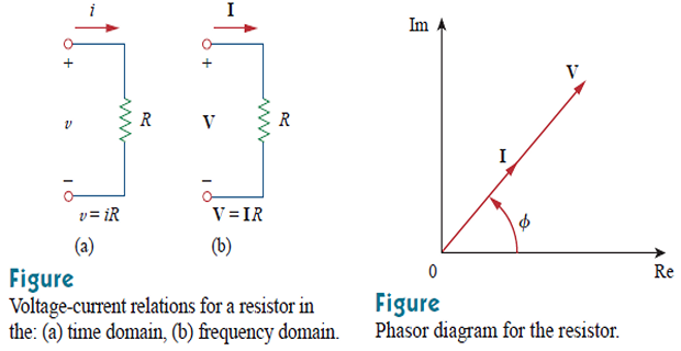
Resistor. Ohm's law \(v = iR\) contains no calculus, so it transforms unchanged:
The phasors differ only in magnitude; there is no phase shift. Voltage and current in a resistor are in phase.
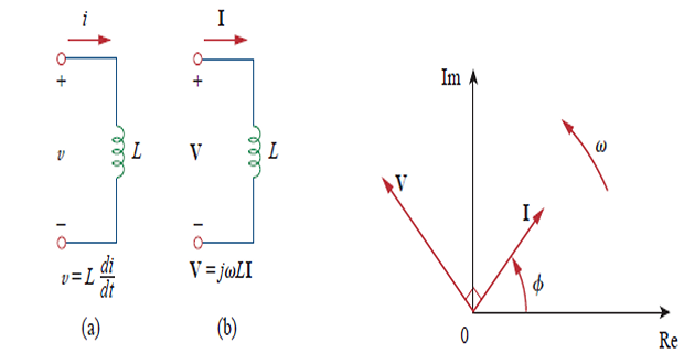
Inductor. Starting from \(v = L\,di/dt\) and replacing the derivative by \(j\omega\):
Since \(j = 1\angle 90^{\circ}\), multiplying by \(j\) advances the phase by 90°. The voltage therefore leads the current by 90° — equivalently, the current lags the voltage by 90°.
Capacitor. Starting from \(i = C\,dv/dt\):
Here the current leads the voltage by 90°, exactly reversing the inductor.
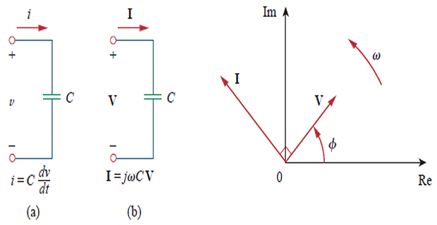
The mnemonic used throughout the English-speaking world is CIVIL: in a Capacitor, I leads V; V leads I in an L. Crude, but it has saved many examination answers.
Impedance and Admittance
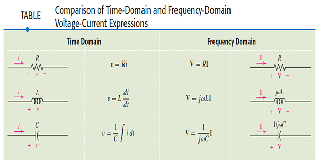
Look at the three relations just derived. Every one has the form "phasor voltage equals something times phasor current". That something is the impedance:
This is Ohm's law in phasor form, and it is the reason every technique of Part 1 survives into AC analysis. Impedance is measured in ohms and represents the opposition a circuit presents to sinusoidal current.
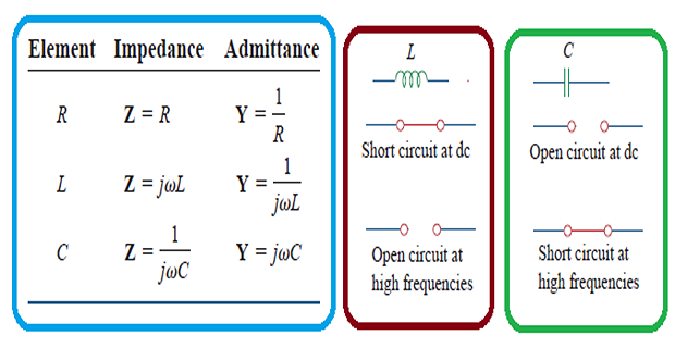
| Element | Impedance \(\mathbf{Z}\) | Admittance \(\mathbf{Y}\) | Phase of \(v\) relative to \(i\) |
|---|---|---|---|
| Resistor | \(R\) | \(\dfrac{1}{R}\) | in phase |
| Inductor | \(j\omega L\) | \(\dfrac{1}{j\omega L}\) | leads by 90° |
| Capacitor | \(\dfrac{1}{j\omega C}\) | \(j\omega C\) | lags by 90° |
Impedance is not a phasor. It is a complex number, but it does not correspond to any sinusoidally varying quantity — it is a ratio of two phasors. This distinction matters: you never write an impedance as a time function.
Note also the frequency dependence. An inductor's impedance \(j\omega L\) grows without limit as frequency rises, so an inductor blocks high frequencies and passes DC. A capacitor's impedance \(1/j\omega C\) does the opposite. At \(\omega = 0\) the inductor becomes a short and the capacitor an open circuit — recovering the DC results of Section 6.8 as a special case.
Being complex, impedance splits into real and imaginary parts:
The real part \(R\) is the resistance, the imaginary part \(X\) the reactance, both in ohms. The sign of \(X\) classifies the circuit:
\(X > 0\) — inductive. The current lags the voltage.
\(X < 0\) — capacitive. The current leads the voltage.
\(X = 0\) — purely resistive. Voltage and current are in phase, which is the resonant condition of Chapter 14.
The reciprocal of impedance is the admittance, in siemens:
where \(G\) is the conductance and \(B\) the susceptance. Rationalising \(1/(R+jX)\) and equating real and imaginary parts gives
A trap worth flagging. \(G\) is not equal to \(1/R\) unless the reactance is zero, and \(B\) is not \(1/X\). The whole complex quantity inverts, not the parts separately. Assuming otherwise is among the most persistent errors in this chapter.
Problem. At \(\omega = 100~\mathrm{rad/s}\), find the impedance of (a) a 20 \(\Omega\) resistor, (b) a 0.1 H inductor, (c) a 500 \(\mu\mathrm{F}\) capacitor. What are their impedances at DC?
Solution.
Note the sign: dividing by \(j\) is the same as multiplying by \(-j\), since \(1/j = -j\). Capacitive reactance is always negative.
At DC (\(\omega = 0\)): the resistor is unchanged at 20 \(\Omega\); the inductor becomes \(j(0)(0.1) = 0\), a short circuit; and the capacitor becomes \(1/j(0)C \to \infty\), an open circuit. The DC replacements of Chapter 6 are simply the \(\omega \to 0\) limit of the impedances.
Problem. A load has \(\mathbf{Z} = 3 + j4~\Omega\). Find \(\left|\mathbf{Z}\right|\), the phase angle, the admittance, and the conductance and susceptance. Is the load inductive or capacitive?
Solution.
Since \(X = +4 > 0\), the load is inductive and the current lags the voltage by 53.13°.
In rectangular form, either by converting the polar result or by rationalising directly:
Observe that \(G = 0.12\) is not \(1/3 = 0.333\), confirming the warning above. Note too that an inductive impedance gives a negative susceptance.
Kirchhoff's Laws in the Frequency Domain
Kirchhoff's laws hold instant by instant in the time domain. Since the phasor transform is linear, they hold in the phasor domain too — and this is what licenses everything that follows.
For KVL, suppose \(v_{1}+v_{2}+\cdots+v_{n} = 0\) around a loop, with every term a sinusoid at the same \(\omega\). Writing each as \(\mathrm{Re}\left(\mathbf{V}_{k}e^{j\omega t}\right)\) and factoring out the common exponential gives
For this to hold at every instant the bracket must vanish, so
and by the identical argument applied to currents at a node,
This is the moment the whole of Part 1 becomes available again. With \(\mathbf{V} = \mathbf{Z}\mathbf{I}\) playing the role of Ohm's law and both Kirchhoff laws intact, every analysis technique from Chapters 2 to 4 carries over unchanged — series and parallel reduction, voltage and current division, wye–delta, nodal and mesh analysis, superposition, source transformation, Thévenin and Norton. The only difference is that the arithmetic is complex.
One thing does not survive. Phasors at different frequencies cannot be added, so a circuit driven at two frequencies must be solved once per frequency and the time-domain results superposed at the end. Chapter 10 returns to this.
Impedance Combinations
Series. The same current flows through each element, so the voltages add:
Parallel. The same voltage appears across each, so the currents add:
For two in parallel, the product-over-sum rule applies as before:
Voltage and current division likewise transfer without change:
Note that the crossover in the current divider — the other impedance on top — is exactly as it was for resistors in Section 2.8.
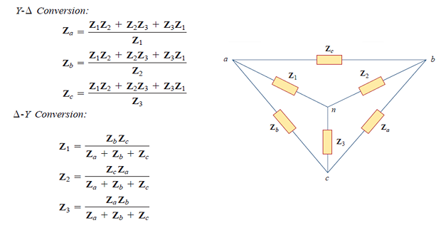
The wye–delta transformation of Section 2.9 also carries over, with \(\mathbf{Z}\) replacing \(R\) throughout:
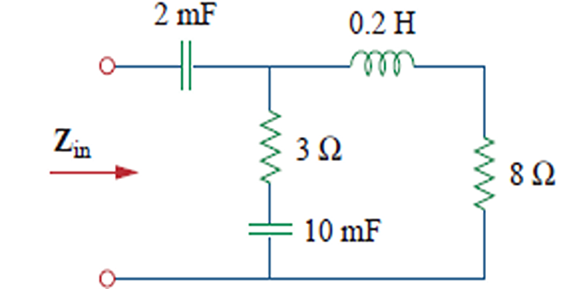
Problem. Find the input impedance of the network below at \(\omega = 50~\mathrm{rad/s}\). A 2 mF capacitor is in series with the parallel combination of (a 3 \(\Omega\) resistor in series with a 10 mF capacitor) and (an 8 \(\Omega\) resistor in series with a 0.2 H inductor).
Solution. Convert each branch to an impedance first:
Now combine \(\mathbf{Z}_{2}\) and \(\mathbf{Z}_{3}\) in parallel by product over sum:
Rationalise by multiplying numerator and denominator by the conjugate of the denominator:
Finally add the series capacitor:
In polar form \(\mathbf{Z}_{\text{in}} = 11.53\angle-73.79^{\circ}~\Omega\). The negative reactance shows the network is net capacitive at this frequency, despite containing an inductor — the series capacitor dominates. That conclusion would change at a different \(\omega\), which is precisely the frequency dependence Chapter 14 exploits.
Problem. A source \(\mathbf{V} = 100\angle 0^{\circ}~\mathrm{V}\) drives a 10 \(\Omega\) resistor in series with a capacitor of reactance \(-j20~\Omega\). Find the current and the voltage across the capacitor, by two methods.
Method 1 — find the current first.
Method 2 — voltage division directly.
Both routes agree. Two observations. The current leads the source voltage by 63.43°, as it must in a net capacitive circuit. And \(\left|\mathbf{V}_{C}\right| = 89.44\) V while the resistor takes \(\left|\mathbf{V}_{R}\right| = \left|10(2+j4)\right| = 44.72\) V — and \(89.44 + 44.72 = 134.2\) V, well over the 100 V supply. In AC circuits, magnitudes do not add; phasors do. Adding \(80-j40\) and \(20+j40\) gives exactly 100 V.
Practical Engineering Applications
A phase shifter delivers an output that is a controlled number of degrees ahead of or behind its input. The simplest is a series RC network with the output taken across one element — and because the impedances are complex, a division of two of them naturally produces a phase angle.
Taking the output across the resistor of a series RC pair:
This is a leading network: the output leads the input by an angle between 0° and 90°, depending on how \(\omega RC\) compares with 1. Taking the output across the capacitor instead gives a lagging network. Cascading identical stages multiplies the shift, which is how RC phase-shift oscillators achieve the 180° they require.
Problem. A series RC network has \(R = 1~\mathrm{k}\Omega\) and \(C = 1~\mu\mathrm{F}\), operating at \(\omega = 1000~\mathrm{rad/s}\), with the output taken across \(R\). Find the magnitude and phase of \(\mathbf{V}_{o}/\mathbf{V}_{i}\).
Solution. The capacitive reactance first:
By voltage division across the resistor:
The output leads by exactly 45° with its amplitude reduced to \(1/\sqrt{2}\) of the input. This is no coincidence: at \(\omega = 1/RC\) the resistance and the reactance are equal in magnitude, which always gives 45° and a factor of \(1/\sqrt{2}\). That frequency is the corner frequency, and the \(0.7071\) is the half-power point that defines bandwidth in Chapter 14.
The Wheatstone bridge of Section 4.9 measured an unknown resistance by balancing two divider ratios. Replacing the resistors by impedances extends the method to inductance and capacitance, and the balance condition takes the same form:
The difference is that this is now a complex equation, so balancing it requires satisfying two real conditions simultaneously — magnitude and phase, or equivalently real and imaginary parts. A practical AC bridge therefore has two adjustable elements, and they interact, so balancing requires alternate adjustment of both.
The named bridges each target a particular quantity: the Maxwell bridge measures inductance by comparing it with a capacitance, the Hay bridge suits high-\(Q\) inductors, and the Schering bridge measures capacitance and dielectric loss. All are the same idea with different arm arrangements, and all inherit the Wheatstone bridge's precision — the supply voltage cancels out, and only a null need be detected.
Summary and Key Formulas
A sinusoid applied to a linear circuit produces a sinusoid of the same frequency; only amplitude and phase change.
A sinusoid is described by amplitude, angular frequency and phase, with \(T = 2\pi/\omega\) and \(\omega = 2\pi f\).
Before comparing phases, convert both sinusoids to positive-amplitude cosines of the same frequency.
A phasor is a complex number carrying the amplitude and phase: \(V_{m}\cos(\omega t + \phi) \leftrightarrow V_{m}\angle\phi\).
Differentiation becomes multiplication by \(j\omega\); integration becomes division by it.
Impedances: \(R\) for a resistor, \(j\omega L\) for an inductor, \(1/j\omega C\) for a capacitor.
Current lags voltage by 90° in an inductor and leads by 90° in a capacitor — CIVIL.
\(\mathbf{Z} = R + jX\); positive \(X\) is inductive, negative capacitive. \(\mathbf{Y} = 1/\mathbf{Z} = G + jB\), and \(G \neq 1/R\) in general.
KVL and KCL hold for phasors, so every technique from Part 1 carries over with complex arithmetic.
Phasors of different frequencies cannot be added; use superposition instead.
| Result | Formula | Notes |
|---|---|---|
| Period and frequency | \(T = \dfrac{2\pi}{\omega}\), \(f = \dfrac{1}{T}\), \(\omega = 2\pi f\) | \(f\) in Hz, \(\omega\) in rad/s |
| Sine to cosine | \(\sin\omega t = \cos\left(\omega t - 90^{\circ}\right)\) | cosine is the reference |
| Negative amplitude | \(-\cos\omega t = \cos\left(\omega t \pm 180^{\circ}\right)\) | normalise before comparing |
| Euler's identity | \(e^{j\phi} = \cos\phi + j\sin\phi\) | basis of the phasor |
| Phasor transform | \(V_{m}\cos(\omega t+\phi) \leftrightarrow V_{m}\angle\phi\) | suppresses \(e^{j\omega t}\) |
| Derivative | \(\dfrac{dv}{dt} \leftrightarrow j\omega\mathbf{V}\) | calculus becomes algebra |
| Integral | \(\displaystyle\int v\,dt \leftrightarrow \dfrac{\mathbf{V}}{j\omega}\) | |
| Ohm's law, phasor form | \(\mathbf{V} = \mathbf{Z}\mathbf{I}\) | |
| Resistor impedance | \(\mathbf{Z}_{R} = R\) | in phase |
| Inductor impedance | \(\mathbf{Z}_{L} = j\omega L\) | current lags 90° |
| Capacitor impedance | \(\mathbf{Z}_{C} = \dfrac{1}{j\omega C} = \dfrac{-j}{\omega C}\) | current leads 90° |
| Impedance components | \(\mathbf{Z} = R + jX = |\mathbf{Z}|\angle\theta\) | \(\theta = \tan^{-1}(X/R)\) |
| Admittance | \(\mathbf{Y} = \dfrac{1}{\mathbf{Z}} = G + jB\) | siemens |
| Conductance | \(G = \dfrac{R}{R^{2}+X^{2}}\) | not \(1/R\) |
| Susceptance | \(B = -\dfrac{X}{R^{2}+X^{2}}\) | |
| Series impedance | \(\mathbf{Z}_{\mathrm{eq}} = \sum \mathbf{Z}_{k}\) | |
| Parallel impedance | \(\mathbf{Y}_{\mathrm{eq}} = \sum \mathbf{Y}_{k}\) | admittances add |
| Voltage division | \(\mathbf{V}_{1} = \dfrac{\mathbf{Z}_{1}}{\mathbf{Z}_{1}+\mathbf{Z}_{2}}\mathbf{V}\) | own impedance on top |
| Current division | \(\mathbf{I}_{1} = \dfrac{\mathbf{Z}_{2}}{\mathbf{Z}_{1}+\mathbf{Z}_{2}}\mathbf{I}\) | other impedance on top |
| AC bridge balance | \(\mathbf{Z}_{x} = \dfrac{\mathbf{Z}_{2}\mathbf{Z}_{3}}{\mathbf{Z}_{1}}\) | two real conditions |
Common Mistakes
Comparing phases without normalising first. Both sinusoids must be positive-amplitude cosines (or both sines) at the same frequency. Skipping this gives an answer wrong by 90° or 180°.
Adding complex numbers in polar form. Magnitudes and angles do not add. Convert to rectangular, add, convert back.
Trusting the calculator's arctangent. It cannot distinguish the second quadrant from the fourth. Check the signs of the real and imaginary parts and add 180° when the real part is negative.
Writing \(G = 1/R\) for a complex impedance. The correct relation is \(G = R/(R^{2}+X^{2})\). The whole quantity inverts, not the parts.
Losing the sign of capacitive reactance. Since \(1/j = -j\), the capacitor impedance is \(-j/\omega C\). Reactance is negative for a capacitor and positive for an inductor.
Adding phasor magnitudes. KVL applies to the phasors themselves. Two series voltages of 80 V and 45 V can perfectly well sum to 100 V.
Adding phasors of different frequencies. The suppressed \(e^{j\omega t}\) factors differ, so the sum is meaningless. Use superposition, one frequency at a time.
Treating a phasor as a function of time. Writing \(\mathbf{V}(t)\) confuses the two domains. The whole point is that time has been removed.
Confusing \(f\) with \(\omega\). A 50 Hz supply has \(\omega = 314.2~\mathrm{rad/s}\). Using 50 for \(\omega\) makes every reactance wrong by a factor of \(2\pi\).
Forgetting that impedance depends on frequency. A network that is inductive at one frequency may be capacitive at another; there is no single answer independent of \(\omega\).
Chapter Review
Work these before opening the answers. Quote phasors in polar form to four significant figures with angles in degrees.
P9.1 For \(v = 20\sin\left(4\pi t - 30^{\circ}\right)~\mathrm{V}\), find \(V_{m}\), \(\omega\), \(f\), \(T\) and \(v\) at \(t = 0.1~\mathrm{s}\).
Show answer
At \(t = 0.1\) s the argument is \(4\pi(0.1) = 0.4\pi~\mathrm{rad} = 72^{\circ}\):\[V_{m} = 20~\mathrm{V}, \quad \omega = 4\pi = 12.57~\mathrm{rad/s}, \quad f = \frac{\omega}{2\pi} = 2~\mathrm{Hz}, \quad T = 0.5~\mathrm{s}\]\[v = 20\sin\left(72^{\circ}-30^{\circ}\right) = 20\sin 42^{\circ} = 13.38~\mathrm{V}\]P9.2 Find the phase relationship between \(v_{1} = 10\cos\left(\omega t + 30^{\circ}\right)\) and \(v_{2} = 8\sin\left(\omega t + 10^{\circ}\right)\).
Show answer
\[v_{2} = 8\cos\left(\omega t + 10^{\circ} - 90^{\circ}\right) = 8\cos\left(\omega t - 80^{\circ}\right)\]\(v_{1}\) leads \(v_{2}\) by 110°.\[30^{\circ} - \left(-80^{\circ}\right) = 110^{\circ}\]P9.3 Transform \(v = 15\sin\left(377t + 25^{\circ}\right)~\mathrm{V}\) to a phasor, and state the supply frequency in hertz.
Show answer
\[v = 15\cos\left(377t + 25^{\circ} - 90^{\circ}\right) = 15\cos\left(377t - 65^{\circ}\right) \;\Longrightarrow\; \mathbf{V} = 15\angle-65^{\circ}~\mathrm{V}\]\[f = \frac{377}{2\pi} = 60.00~\mathrm{Hz}\]P9.4 Given \(\mathbf{V} = 30\angle-90^{\circ}~\mathrm{V}\) at \(\omega = 60~\mathrm{rad/s}\), write \(v(t)\) in both cosine and sine form.
Show answer
since \(\cos(x-90^{\circ}) = \sin x\).\[v(t) = 30\cos\left(60t - 90^{\circ}\right)~\mathrm{V} = 30\sin 60t~\mathrm{V}\]P9.5 At \(f = 60~\mathrm{Hz}\), find the impedances of a 50 \(\Omega\) resistor, a 0.2 H inductor and a 100 \(\mu\mathrm{F}\) capacitor.
Show answer
\[\omega = 2\pi(60) = 377~\mathrm{rad/s}\]\[\mathbf{Z}_{R} = 50~\Omega, \qquad \mathbf{Z}_{L} = j(377)(0.2) = j75.40~\Omega\]\[\mathbf{Z}_{C} = \frac{-j}{(377)\left(100\times10^{-6}\right)} = -j26.53~\Omega\]P9.6 Find the admittance of \(\mathbf{Z} = 8 - j6~\Omega\), and state whether the load is inductive or capacitive.
Show answer
\[\left|\mathbf{Z}\right| = \sqrt{64+36} = 10~\Omega\]Since \(X = -6 < 0\) the load is capacitive, and the current leads the voltage.\[\mathbf{Y} = \frac{8+j6}{100} = 0.0800 + j0.0600~\mathrm{S}\]P9.7 Find \(\mathbf{Z}_{\mathrm{eq}}\) for \(\left(4+j3\right)~\Omega\) in series with \(\left(2-j5\right)~\Omega\), in polar form.
Show answer
\[\mathbf{Z}_{\mathrm{eq}} = \left(4+2\right) + j\left(3-5\right) = 6 - j2~\Omega\]\[\left|\mathbf{Z}\right| = \sqrt{36+4} = 6.325~\Omega, \qquad \theta = \tan^{-1}\frac{-2}{6} = -18.43^{\circ}\]P9.8 An inductor of reactance \(j10~\Omega\) is in parallel with a capacitor of reactance \(-j5~\Omega\). Find the equivalent impedance and comment.
Show answer
The combination is capacitive, with a reactance larger in magnitude than either element. Parallel reactances of opposite sign can produce this — and if the two were equal in magnitude the denominator would vanish, giving infinite impedance. That is parallel resonance, and Chapter 14 treats it fully.\[\mathbf{Z}_{\mathrm{eq}} = \frac{\left(j10\right)\left(-j5\right)}{j10 - j5} = \frac{50}{j5} = -j10~\Omega\]P9.9 A source \(120\angle 0^{\circ}~\mathrm{V}\) drives 30 \(\Omega\) in series with \(j40~\Omega\). Find the voltage across the inductor.
Show answer
\[\mathbf{V}_{L} = \frac{j40}{30+j40}\left(120\angle 0^{\circ}\right) = \frac{40\angle 90^{\circ}}{50\angle 53.13^{\circ}}\left(120\right)\]\[\mathbf{V}_{L} = 96.00\angle 36.87^{\circ}~\mathrm{V}\]P9.10 For the phase shifter of Worked Example 9.9, what happens to the phase shift as \(\omega\) becomes very large, and very small?
Show answer
With the output across \(R\), \(\mathbf{V}_o/\mathbf{V}_i = j\omega RC/(1+j\omega RC)\).
As \(\omega \to \infty\) the ratio tends to 1, so the shift tends to 0° and the output equals the input — the capacitor becomes a short.
As \(\omega \to 0\) the ratio tends to \(j\omega RC\), so the shift tends to +90° while the amplitude falls to zero. The full 90° is approached only where there is no output left to shift — a limitation of every single-stage RC network.
MCQ 1. A 50 Hz supply has an angular frequency of:
(a) 50 rad/s (b) 157.1 rad/s (c) 314.2 rad/s (d) 377 rad/sShow answer
(c) 314.2 rad/s. \(\omega = 2\pi(50)\). Option (d) corresponds to 60 Hz.MCQ 2. The phasor for \(10\sin\left(\omega t + 20^{\circ}\right)\) is:
(a) \(10\angle 20^{\circ}\) (b) \(10\angle-70^{\circ}\) (c) \(10\angle 110^{\circ}\) (d) \(10\angle-20^{\circ}\)Show answer
(b) \(10\angle-70^{\circ}\). Converting, \(10\sin(\omega t+20^{\circ}) = 10\cos(\omega t - 70^{\circ})\). Option (a) is the trap.MCQ 3. In an inductor, the current:
(a) leads the voltage by 90° (b) lags the voltage by 90° (c) is in phase with the voltage (d) lags by 45°Show answer
(b) lags by 90°. Recall CIVIL: V leads I in an L.MCQ 4. The impedance of a capacitor is:
(a) \(j\omega C\) (b) \(\omega C\) (c) \(\dfrac{-j}{\omega C}\) (d) \(\dfrac{j}{\omega C}\)Show answer
(c) \(-j/\omega C\), since \(1/(j\omega C) = -j/\omega C\). Option (a) is the admittance.MCQ 5. An impedance \(\mathbf{Z} = 5 - j5~\Omega\) is:
(a) inductive (b) capacitive (c) purely resistive (d) resonantShow answer
(b) capacitive, since the reactance is negative. The current leads by 45°.MCQ 6. For \(\mathbf{Z} = 6 + j8~\Omega\), the conductance \(G\) is:
(a) 0.1667 S (b) 0.06 S (c) 0.1 S (d) 0.08 SShow answer
(b) 0.06 S. \(G = R/(R^{2}+X^{2}) = 6/100\). Option (a) is the trap \(1/R\).MCQ 7. In the phasor domain, differentiation corresponds to:
(a) division by \(j\omega\) (b) multiplication by \(j\omega\) (c) multiplication by \(\omega\) (d) no changeShow answer
(b) multiplication by \(j\omega\). Integration divides by it.MCQ 8. Two impedances of 3 \(\Omega\) and \(j4~\Omega\) in series give a magnitude of:
(a) 7 \(\Omega\) (b) 5 \(\Omega\) (c) 12 \(\Omega\) (d) 1 \(\Omega\)Show answer
(b) 5 \(\Omega\). \(\left|3+j4\right| = \sqrt{9+16}\). Option (a) adds magnitudes, which is wrong.MCQ 9. Phasors may be added only if the sinusoids have the same:
(a) amplitude (b) phase (c) frequency (d) waveformShow answer
(c) frequency. Otherwise the suppressed \(e^{j\omega t}\) factors differ and the sum is meaningless.MCQ 10. At \(\omega = 0\), an inductor behaves as:
(a) an open circuit (b) a short circuit (c) a resistor (d) a capacitorShow answer
(b) a short circuit, since \(\mathbf{Z}_{L} = j\omega L \to 0\) — recovering the DC result of Chapter 6.
Why is the sinusoid the only waveform that passes through a linear circuit unchanged in shape? What would go wrong if we tried to build a "phasor" for a square wave?
A phasor is often described as a rotating vector, yet it is defined as a fixed complex number. Reconcile these two descriptions.
Explain why impedance, although complex, is not a phasor. What would it even mean to write \(\mathbf{Z}(t)\)?
In Worked Example 9.8 the two element voltages have magnitudes 89.44 V and 44.72 V across a 100 V supply. Explain why this does not violate KVL.
The DC results of Chapter 6 — capacitor open, inductor short — emerge as the \(\omega\to0\) limit of the impedances. What is the corresponding statement as \(\omega\to\infty\), and what does it imply for filtering?
An AC bridge requires two adjustments where a Wheatstone bridge needs one. Explain why, in terms of what "balance" means for a complex equation.
The machinery is now in place but has been applied only to single elements and simple series–parallel combinations. Chapter 10 turns it loose on complete circuits.
Nodal and mesh analysis, superposition, source transformation, Thévenin and Norton — all return, unchanged in structure, with impedances in place of resistances and complex arithmetic in place of real. Nothing new has to be learned, which is precisely the point: the effort invested in Part 1 pays for itself twice over.
Chapter 11 then asks what all this means for power, where the phase angle between voltage and current turns out to matter enormously — a 90° phase shift means an element that consumes no net energy at all, however large the voltage and current across it. That observation leads to reactive power, power factor, and the economics of the electricity supply.