- Apply the three-step methodology: transform to the frequency domain, solve, transform back.
- Perform nodal analysis on phasor circuits, including those with dependent sources and supernodes.
- Perform mesh analysis on phasor circuits, including supermeshes.
- Use superposition for circuits with several sources.
- Handle circuits whose sources operate at different frequencies, where phasors cannot be combined.
- Apply source transformation between voltage and current sources with impedances.
- Find the Thévenin and Norton equivalents of an AC network, including when dependent sources are present.
- Analyse operational amplifier circuits driven by sinusoidal sources.
Introduction
Chapter 9 built the machinery: phasors, impedance, and the proof that Kirchhoff's laws survive the transform. This chapter puts it to work, and it is the shortest-to-learn chapter in the book — because there is almost nothing new in it.
The claim made at the end of Chapter 9 was that every analysis technique from Part 1 carries over to AC circuits unchanged. That claim is now cashed in. Nodal analysis, mesh analysis, supernodes, supermeshes, superposition, source transformation, Thévenin and Norton: all of them work exactly as before. The equations have the same structure, the procedures have the same steps, and the checks are the same checks.
What changes is the arithmetic. Real numbers become complex, which means more careful bookkeeping and a good deal more use of the calculator's polar–rectangular conversion. It also means the answers carry phase information, and interpreting that phase is where the physical insight lies.
The Analysis Methodology
Every problem in this chapter follows the same three steps.
Transform the circuit to the phasor domain. Replace every source by its phasor, and every element by its impedance at the source frequency \(\omega\). Resistors keep their value; inductors become \(j\omega L\); capacitors become \(1/j\omega C\).
Solve the problem using any circuit technique — nodal, mesh, superposition, Thévenin. The arithmetic is complex; the method is unchanged.
Transform the answer back to the time domain, if a time function was asked for. A phasor \(\mathbf{I} = I_{m}\angle\theta\) at frequency \(\omega\) becomes \(i(t) = I_{m}\cos\left(\omega t + \theta\right)\).

Two points of practice. Step 1 requires \(\omega\), so read it from the source before doing anything else — an impedance is meaningless without a frequency. And step 3 is often forgotten: if the question asks for \(i(t)\) rather than \(\mathbf{I}\), a phasor is not an answer.
Since this chapter's methods produce simultaneous complex equations, a calculator or software able to solve them directly is a considerable help. Solving \(2\times2\) complex systems by hand using Cramer's rule, as in Section 3.6, remains entirely practical and is what the worked examples do.
Nodal Analysis
Since KCL holds for phasors, nodal analysis proceeds exactly as in Section 3.2. Choose a reference node, assign phasor node voltages, and write KCL at each non-reference node with every branch current expressed as a potential difference divided by an impedance.
Dependent sources are handled as in Section 3.8: treat them as ordinary sources when writing the equations, then add a constraint expressing the controlling variable in terms of the node voltages.
Problem. A current source \(5\angle 0^{\circ}~\mathrm{A}\) feeds node 1. From node 1, a 10 \(\Omega\) resistor runs to ground and a \(j5~\Omega\) inductor runs to node 2; from node 2 a \(-j10~\Omega\) capacitor runs to ground. Find \(\mathbf{V}_{1}\) and \(\mathbf{V}_{2}\).
Solution. KCL at node 2 first, since it has only two branches:
Multiplying through by \(j10\) gives \(2\left(\mathbf{V}_{1}-\mathbf{V}_{2}\right) = -\mathbf{V}_{2}\), hence
KCL at node 1, substituting this result:
Since \(1/j = -j\), the second term is \(+j\mathbf{V}_{1}/5\):
Check. Substituting back into node 1: \(\left(10-j20\right)/10 = 1-j2\), and \(\left(-10+j20\right)/j5 = 4+j2\), summing to exactly \(5\) \(\checkmark\). Note that both node voltages share the same phase angle here, which happens because the ratio between them turned out purely real.
Problem. In a circuit operating at \(\omega = 4~\mathrm{rad/s}\), a 20 V source drives node 1 through 10 \(\Omega\). Node 1 connects to ground through \(-j2.5~\Omega\) and to node 2 through \(j4~\Omega\); node 2 connects to ground through \(j2~\Omega\). A dependent current source \(2\mathbf{I}_{x}\) feeds node 2, where \(\mathbf{I}_{x}\) is the current in the \(-j2.5~\Omega\) branch. Find \(i_{x}(t)\).
Solution. KCL at node 1:
KCL at node 2, with the constraint \(\mathbf{I}_{x} = \mathbf{V}_{1}/(-j2.5)\) substituted immediately:
In matrix form:
From the second equation \(\mathbf{V}_{2} = -11\mathbf{V}_{1}/15\). Substituting into the first:
Finally the controlling current itself:
Step 3 of the methodology has been applied: the question asked for \(i_{x}(t)\), so \(\omega = 4\) is reinstated and the phasor becomes a cosine.

Supernodes
A voltage source between two non-reference nodes requires a supernode, exactly as in Section 3.3. Enclose the source and both nodes, write KCL for the branches crossing the boundary, and add the source constraint.
Problem. A 3 A current source feeds a supernode. Node 1 connects to ground through \(-j3~\Omega\); node 2 connects to ground through \(j6~\Omega\) and through 12 \(\Omega\). A voltage source of \(10\angle 45^{\circ}~\mathrm{V}\) joins node 2 to node 1. Find \(\mathbf{V}_{1}\) and \(\mathbf{V}_{2}\).
Solution. KCL across the supernode boundary — the source itself is inside and does not appear:
The constraint supplied by the source:
Writing \(10\angle45^{\circ} = 7.071 + j7.071\) and substituting, then collecting terms in \(\mathbf{V}_{2}\):
Note that the final addition had to be performed in rectangular form: \(\left(1.545 - j31.37\right) + \left(7.071 + j7.071\right) = 8.616 - j24.30\). Adding the polar magnitudes would have been meaningless.

Mesh Analysis
KVL holds for phasors, so mesh analysis transfers likewise. Assign mesh currents, conventionally all clockwise, and write KVL around each mesh with element voltages expressed as \(\mathbf{Z}\mathbf{I}\). For an impedance shared between meshes \(j\) and \(k\), the drop seen from mesh \(j\) is \(\mathbf{Z}\left(\mathbf{I}_{j}-\mathbf{I}_{k}\right)\) — the own mesh current first, exactly as in Section 3.4.
The by-inspection method of Section 3.6 also survives, with the resistance matrix becoming an impedance matrix. With only independent sources present it remains symmetric, which is as useful an error check here as it was there.
Problem. A \(30\angle 0^{\circ}~\mathrm{V}\) source drives mesh 1, which contains a 6 \(\Omega\) resistor and shares a \(j8~\Omega\) inductor with mesh 2. Mesh 2 contains the shared \(j8~\Omega\) and a \(-j4~\Omega\) capacitor. Find both mesh currents and the current in the shared branch.
Solution. KVL around mesh 2, which has no source:
KVL around mesh 1, substituting:
The shared branch carries the difference, taken in the direction of \(\mathbf{I}_{1}\):
Check. Substituting into mesh 1: \(6(1.8+j2.4) + j8(-1.8-j2.4) = 10.8 + j14.4 - j14.4 + 19.2 = 30\) \(\checkmark\). Note that \(\mathbf{I}_{2}\) is larger than \(\mathbf{I}_{1}\), which is possible because mesh 2 contains the near-cancelling pair \(j8\) and \(-j4\) and is close to resonance.

Supermeshes
A current source shared by two meshes requires a supermesh, as in Section 3.5: take KVL around the combined loop excluding the branch containing the source, and supply the constraint \(\mathbf{I}_{j}-\mathbf{I}_{k} = \mathbf{I}_{s}\).
A source belonging to one mesh alone is easier still: that mesh current is simply known, and no KVL equation is written for it. In the four-mesh circuit below, two of the four unknowns are fixed this way:
Four equations, of which two are constraints rather than KVL statements. Solving gives \(\mathbf{I}_{1} = 3.618\angle 274.5^{\circ}~\mathrm{A}\), and the voltage across the \(-j2~\Omega\) element follows:

Superposition
Superposition applies to phasor circuits for the same reason it applied to resistive ones: linearity. Deactivate all independent sources but one, solve, and repeat; then sum the partial responses. The deactivation rules are unchanged — voltage sources become short circuits, current sources become open circuits, and dependent sources are never deactivated.
For a circuit whose sources all share one frequency, superposition is legitimate but rarely economical: it means solving several circuits instead of one. Its indispensable role appears in the next section, where the sources have different frequencies and no other method will do.
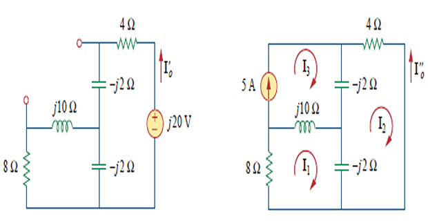
Problem. A \(20\angle 0^{\circ}~\mathrm{V}\) source drives a node through a 5 \(\Omega\) resistor. A \(4\angle 90^{\circ}~\mathrm{A}\) current source also feeds the same node, and a \(-j5~\Omega\) capacitor connects the node to ground. Find the node voltage by superposition.
Part 1 — voltage source alone. Open-circuit the current source. What remains is a voltage divider:
Part 2 — current source alone. Short-circuit the voltage source. The 5 \(\Omega\) and \(-j5~\Omega\) are now in parallel:
Sum.
A striking result: the two contributions have equal magnitude 14.14 V but opposite phase angles of \(\mp45^{\circ}\), and their imaginary parts cancel exactly. The total is purely real. This is why phasors must be summed rather than magnitudes — adding \(14.14 + 14.14 = 28.28\) V would be wrong by 40 %.
Sources at Different Frequencies
Here superposition is not merely convenient but necessary. Recall from Section 9.5 that phasors suppress the factor \(e^{j\omega t}\). If two sources have different \(\omega\), the suppressed factors differ, and their phasors cannot be added — the sum would be meaningless.
Worse, the impedances differ too. An inductor presents \(j\omega L\), which is not the same element at 50 rad/s as at 500 rad/s. There is no single frequency-domain circuit that represents the problem.
The procedure:
Take one frequency at a time, deactivating sources at all other frequencies.
Draw the frequency-domain circuit for that frequency, recomputing every impedance.
Solve, and immediately transform the answer back to the time domain.
Repeat for each frequency, and add the time-domain results.
The addition happens in step 4, in the time domain, where sinusoids of different frequencies coexist perfectly happily. A DC source counts as a separate "frequency" with \(\omega = 0\), at which inductors are shorts and capacitors open circuits.
One consequence worth noting for Chapter 11: powers from different frequencies do add directly, because the cross terms average to zero over time. But voltages and currents must be combined as time functions.
Problem. A series circuit of \(R = 3~\Omega\) and \(L = 0.8~\mathrm{H}\) is driven by two sources in series: a 10 V DC source and a source \(5\cos 5t~\mathrm{V}\). Find the total current \(i(t)\).
Part 1 — the DC source, \(\omega = 0\). Short the AC source. At DC the inductor is a short circuit:
Part 2 — the AC source, \(\omega = 5~\mathrm{rad/s}\). Short the DC source and recompute the impedance at this frequency:
Transform back before combining:
Total. Adding in the time domain:
This is the answer, and it cannot be written as a single phasor — it is a DC level with a sinusoidal ripple riding on it. Attempting to add \(3.333\angle 0^{\circ}\) to \(1\angle-53.13^{\circ}\) would produce a number, but that number would mean nothing.
The physical picture is worth noting: the inductor passes DC freely (it is a short at \(\omega=0\)) but impedes the AC component, whose amplitude is reduced by the factor \(3/5\) relative to what a purely resistive circuit would give. This is exactly the smoothing action of a choke in a power supply.
Source Transformation
The transformation of Section 4.4 carries over directly, with impedance replacing resistance:
A voltage source \(\mathbf{V}_{s}\) in series with \(\mathbf{Z}_{s}\) is indistinguishable, at its terminals, from a current source \(\mathbf{V}_{s}/\mathbf{Z}_{s}\) in parallel with the same \(\mathbf{Z}_{s}\). The current-source arrow points towards what was the positive terminal, and an ideal source with no series or parallel impedance cannot be transformed.
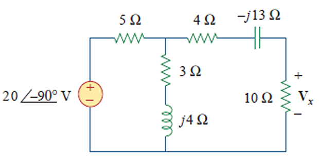
Problem. A source \(20\angle 90^{\circ}~\mathrm{V}\) in series with 5 \(\Omega\) feeds a network in which a \(\left(3+j4\right)~\Omega\) branch appears in parallel with the 5 \(\Omega\). The result drives a 10 \(\Omega\) resistor through a \(\left(4-j13\right)~\Omega\) branch. Find \(\mathbf{V}_{x}\) across the 10 \(\Omega\).
Solution. Transform the source to its current form:
Combine the 5 \(\Omega\) with the \(\left(3+j4\right)~\Omega\) branch in parallel:
Now transform back to a voltage source, taking the reference direction into account so that the equivalent source is
Finally apply voltage division across the remaining series chain:
Source transformation earned its place here: it replaced a parallel branch and a source with a single series pair, avoiding simultaneous equations entirely. As in Chapter 4, its value is greatest when it lets two dissimilar sources be merged or a network be collapsed into a chain.
Thévenin and Norton Equivalents
The two most useful theorems of Chapter 4 transfer intact. Any linear two-terminal AC network can be replaced by
a voltage source \(\mathbf{V}_{Th}\) in series with an impedance \(\mathbf{Z}_{Th}\), or
a current source \(\mathbf{I}_{N}\) in parallel with the same impedance,
related by the same conversion as before:
The methods for finding \(\mathbf{Z}_{Th}\) are those of Sections 4.5 and 4.7: deactivate the independent sources and reduce, when only independent sources are present; otherwise use \(\mathbf{V}_{oc}/\mathbf{I}_{sc}\) or apply a test source.
One difference matters. \(\mathbf{Z}_{Th}\) is complex and frequency-dependent. A network's Thévenin equivalent is valid only at the frequency for which it was computed — change \(\omega\) and both \(\mathbf{V}_{Th}\) and \(\mathbf{Z}_{Th}\) change with it.
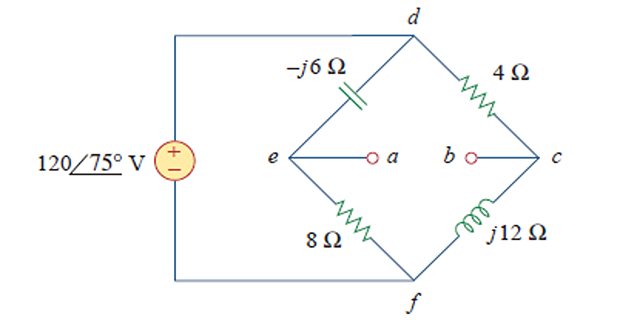
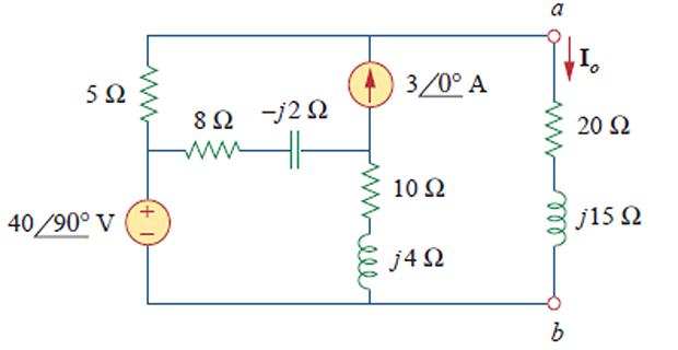
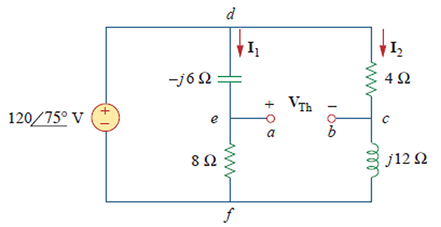
Problem. Obtain the Thévenin equivalent at terminals \(a\)–\(b\) of a circuit driven by \(120\angle 75^{\circ}~\mathrm{V}\), in which an 8 \(\Omega\) resistor is in parallel with \(-j6~\Omega\) forming one branch, and a 4 \(\Omega\) resistor is in parallel with \(j12~\Omega\) forming another.
Step 1 — \(\mathbf{Z}_{Th}\). Deactivate the source (short it) and reduce each parallel pair:
The equivalent is net capacitive at this frequency, despite the network containing an inductor.
Step 2 — \(\mathbf{V}_{Th}\). With the terminals open, the two branch currents are
and KVL across the terminals gives \(\mathbf{V}_{Th} = 4\mathbf{I}_{2} + j6\mathbf{I}_{1}\):
Note that the two contributions had to be converted to rectangular form before adding — their magnitudes, 37.95 and 72, sum to nothing meaningful.
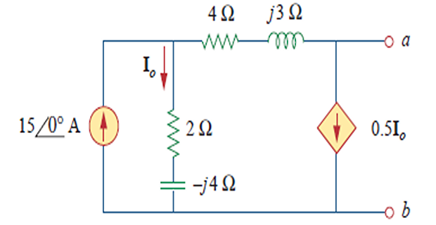
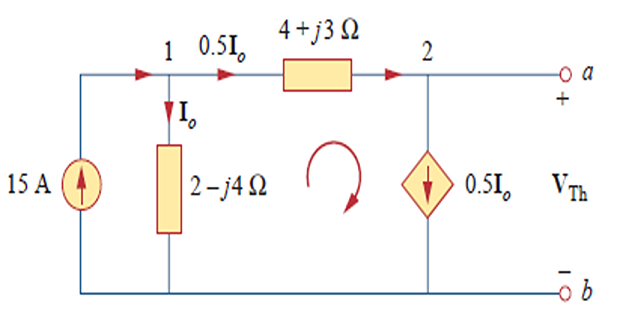
Problem. A network contains a 15 A source feeding a node, a dependent current source \(0.5\mathbf{I}_{o}\), and impedances \(\left(2-j4\right)~\Omega\) and \(\left(4+j3\right)~\Omega\), where \(\mathbf{I}_{o}\) is the current in the \(\left(2-j4\right)\) branch. Find the Thévenin equivalent.
Step 1 — \(\mathbf{V}_{Th}\). With the terminals open, KCL at the node gives
Applying KVL to reach the terminals:
Step 2 — \(\mathbf{Z}_{Th}\) by the test-source method. Deactivate the 15 A independent source but keep the dependent source, and inject a test current \(\mathbf{I}_{s} = 3~\mathrm{A}\):
The test-source method of Section 4.7 works unchanged in the frequency domain. As there, the dependent source is never deactivated — only the independent one.
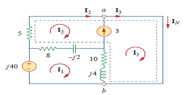
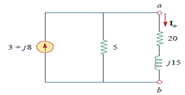
Problem. A network has \(\mathbf{Z}_{N} = 5~\Omega\), and mesh analysis of the short-circuited network yields \(\mathbf{I}_{N} = \left(3+j8\right)~\mathrm{A}\). Find the current \(\mathbf{I}_{o}\) delivered to a load of \(\left(20+j15\right)~\Omega\).
Solution. With the Norton equivalent driving the load, current division applies:
Dividing numerator and denominator by 5:
Note the crossover in the current-divider rule — the source impedance appears in the numerator, matching the pattern of Section 2.8. As always, the division was done in polar form and the subtraction of angles handled separately from the ratio of magnitudes.
Applications: Op Amp AC Circuits
The two golden rules of Chapter 5 depended only on the ideal op-amp assumptions and negative feedback, neither of which involves frequency. They therefore apply unchanged to phasor circuits:
The inverting amplifier's gain becomes a ratio of impedances rather than resistances:
Since the ratio is now complex, the circuit provides both gain and phase shift, and both vary with frequency. This single observation is the foundation of the active filter, and Chapter 14 develops it fully.
The integrator and differentiator of Section 6.9 are special cases. With \(\mathbf{Z}_{f} = 1/j\omega C\) and \(\mathbf{Z}_{1} = R\) the gain is \(-1/j\omega RC\), which falls as frequency rises — the frequency-domain signature of integration.
Problem. An inverting amplifier has \(\mathbf{Z}_{1} = 10~\mathrm{k}\Omega\) and a feedback network consisting of a 10 \(\mathrm{k}\Omega\) resistor in parallel with a 10 nF capacitor. Find the gain at \(\omega = 10^{4}~\mathrm{rad/s}\).
Solution. The capacitor's impedance at this frequency:
The feedback impedance is the parallel combination:
The gain magnitude is 0.7071 with a phase shift of 135°. That 135° is the 180° of the inverting configuration reduced by the 45° that the RC network contributes — and the 0.7071 is the same half-power factor met in Example 9.9, arising for the same reason: at \(\omega = 1/RC\) the resistance and reactance are equal.
At low frequencies the capacitor is an open circuit and the gain approaches the DC value of \(-1\); at high frequencies the capacitor shorts \(\mathbf{Z}_{f}\) and the gain falls towards zero. The circuit is a low-pass filter with gain, and this frequency-dependent behaviour is exactly what Chapter 14 will characterise.
An oscillator produces a sinusoid with no sinusoidal input at all, and the phase relationships of this chapter explain how. The requirements, known as the Barkhausen criteria, are that a loop consisting of an amplifier and a frequency-selective feedback network must have a total loop gain of at least unity in magnitude and a total phase shift of exactly 0° (or 360°) at the desired frequency.
In an RC phase-shift oscillator the amplifier is an inverting stage contributing 180°, and three cascaded RC sections contribute the remaining 180° at one particular frequency — each section supplying roughly 60°, as Section 9.10 showed a single section can. In a Wien-bridge oscillator the amplifier is non-inverting, contributing 0°, and a series–parallel RC network provides zero phase shift only at \(\omega = 1/RC\), where its attenuation is exactly \(1/3\) — so the amplifier gain must be set to 3.
Both designs rest entirely on the observation that a network's phase shift varies with frequency, and that there is generally exactly one frequency at which a required shift is achieved.
Summary and Key Formulas
The methodology is: transform to the frequency domain, solve by any method, transform back if a time function is required.
Nodal analysis, mesh analysis, supernodes and supermeshes work exactly as in Chapter 3, with impedances and complex arithmetic.
Dependent sources require a constraint equation and are never deactivated.
Superposition applies, with voltage sources shorted and current sources opened.
For sources at different frequencies, superposition is compulsory: solve at each frequency separately, recomputing every impedance, and add the results in the time domain.
Source transformation uses \(\mathbf{V}_{s} = \mathbf{Z}_{s}\mathbf{I}_{s}\).
Thévenin and Norton equivalents exist for any linear AC network, with \(\mathbf{Z}_{Th} = \mathbf{V}_{oc}/\mathbf{I}_{sc}\) and both parameters valid only at the frequency for which they were found.
Op-amp golden rules hold unchanged, so the inverting gain becomes \(-\mathbf{Z}_{f}/\mathbf{Z}_{1}\) — complex, and frequency-dependent.
| Result | Formula | Notes |
|---|---|---|
| Branch current, nodal | \(\mathbf{I} = \dfrac{\mathbf{V}_{j}-\mathbf{V}_{k}}{\mathbf{Z}}\) | as in Chapter 3 |
| Shared branch, mesh | \(\mathbf{Z}\left(\mathbf{I}_{j}-\mathbf{I}_{k}\right)\) | own mesh current first |
| Supernode constraint | \(\mathbf{V}_{j}-\mathbf{V}_{k} = \mathbf{V}_{s}\) | plus KCL across the boundary |
| Supermesh constraint | \(\mathbf{I}_{j}-\mathbf{I}_{k} = \mathbf{I}_{s}\) | plus KVL round the outer loop |
| Superposition | \(\mathbf{V} = \mathbf{V}_{a}+\mathbf{V}_{b}+\cdots\) | same frequency only |
| Different frequencies | \(v(t) = v_{1}(t)+v_{2}(t)+\cdots\) | add in the time domain |
| Source transformation | \(\mathbf{V}_{s} = \mathbf{Z}_{s}\mathbf{I}_{s}\) | finite non-zero \(\mathbf{Z}_{s}\) |
| Thévenin voltage | \(\mathbf{V}_{Th} = \mathbf{V}_{oc}\) | terminals open |
| Norton current | \(\mathbf{I}_{N} = \mathbf{I}_{sc}\) | terminals shorted |
| Equivalence | \(\mathbf{V}_{Th} = \mathbf{Z}_{N}\mathbf{I}_{N}\), \(\mathbf{Z}_{Th} = \mathbf{Z}_{N}\) | frequency-dependent |
| \(\mathbf{Z}_{Th}\) by ratio | \(\mathbf{Z}_{Th} = \dfrac{\mathbf{V}_{oc}}{\mathbf{I}_{sc}}\) | always valid |
| \(\mathbf{Z}_{Th}\) by test source | \(\mathbf{Z}_{Th} = \dfrac{\mathbf{V}_{s}}{\mathbf{I}_{s}}\) | independent sources off |
| Inverting op amp | \(\dfrac{\mathbf{V}_{o}}{\mathbf{V}_{i}} = -\dfrac{\mathbf{Z}_{f}}{\mathbf{Z}_{1}}\) | gain and phase shift |
| Phasor to time domain | \(I_{m}\angle\theta \to I_{m}\cos\left(\omega t+\theta\right)\) | do not omit this step |
Common Mistakes
Adding phasors from sources at different frequencies. The suppressed \(e^{j\omega t}\) factors differ, and so do all the impedances. Solve separately and add the time functions.
Leaving the answer as a phasor when a time function was asked for. Step 3 of the methodology exists for a reason. \(\mathbf{I} = 5\angle 30^{\circ}\) is not an answer to "find \(i(t)\)".
Computing impedances without checking \(\omega\). An impedance is meaningless without a frequency, and a circuit with two sources has two sets of impedances.
Adding complex quantities in polar form. Convert to rectangular first. This costs more keystrokes in AC analysis than any other single habit.
Deactivating a dependent source. Only independent sources are ever deactivated — in superposition, and when finding \(\mathbf{Z}_{Th}\).
Adding magnitudes instead of phasors. In Example 10.5 two contributions of 14.14 V sum to 20 V, not 28.28 V.
Forgetting that \(1/j = -j\). This sign error propagates silently through an entire solution.
Assuming a Thévenin equivalent holds at all frequencies. It holds at one frequency only.
Reversing the order in a shared mesh branch. From mesh \(j\) the drop is \(\mathbf{Z}\left(\mathbf{I}_{j}-\mathbf{I}_{k}\right)\), exactly as in Chapter 3.
Losing track of which angle unit is in use. Phasor angles are conventionally in degrees; the argument \(\omega t\) is in radians. Convert deliberately, not accidentally.
Chapter Review
Work these before opening the answers. Quote phasors in polar form to four significant figures, and give time functions where asked.
P10.1 A \(4\angle 0^{\circ}~\mathrm{A}\) source feeds a node connected to ground through a 5 \(\Omega\) resistor and a \(j5~\Omega\) inductor in parallel. Find the node voltage.
Show answer
\[\mathbf{Z}_{p} = \frac{5\left(j5\right)}{5+j5} = 2.5 + j2.5~\Omega\]\[\mathbf{V} = \left(4\right)\left(2.5+j2.5\right) = 10 + j10~\mathrm{V} = 14.14\angle 45^{\circ}~\mathrm{V}\]P10.2 A \(100\angle 0^{\circ}~\mathrm{V}\) source drives a single loop containing 6 \(\Omega\) and \(j8~\Omega\). Find the current, and state whether it leads or lags.
Show answer
The current lags by 53.13°, as it must in an inductive circuit.\[\mathbf{I} = \frac{100}{6+j8} = \frac{100\left(6-j8\right)}{100} = 6 - j8~\mathrm{A} = 10\angle-53.13^{\circ}~\mathrm{A}\]P10.3 A series circuit of 4 \(\Omega\) and 1 H is driven by a 12 V DC source in series with \(6\cos 4t~\mathrm{V}\). Find \(i(t)\).
Show answer
DC: the inductor is a short, so \(I_{1} = 12/4 = 3~\mathrm{A}\).
AC at \(\omega = 4\):\[\mathbf{Z} = 4 + j4 = 5.657\angle 45^{\circ}~\Omega, \qquad \mathbf{I}_{2} = \frac{6}{5.657\angle 45^{\circ}} = 1.061\angle-45^{\circ}~\mathrm{A}\]\[i(t) = 3 + 1.061\cos\left(4t - 45^{\circ}\right)~\mathrm{A}\]P10.4 Convert a \(20\angle 0^{\circ}~\mathrm{V}\) source in series with \(\left(4+j3\right)~\Omega\) into its Norton form.
Show answer
in parallel with \(\left(4+j3\right)~\Omega\).\[\mathbf{I}_{s} = \frac{20}{4+j3} = \frac{20\left(4-j3\right)}{25} = 3.2 - j2.4~\mathrm{A} = 4\angle-36.87^{\circ}~\mathrm{A}\]P10.5 A \(50\angle 0^{\circ}~\mathrm{V}\) source in series with 10 \(\Omega\) feeds terminals \(a\)–\(b\), across which a \(-j10~\Omega\) capacitor is connected. Find the Thévenin equivalent.
Show answer
\[\mathbf{V}_{Th} = \frac{-j10}{10-j10}\left(50\right) = 25 - j25~\mathrm{V} = 35.36\angle-45^{\circ}~\mathrm{V}\]\[\mathbf{Z}_{Th} = 10\parallel\left(-j10\right) = \frac{10\left(-j10\right)}{10-j10} = 5 - j5~\Omega\]P10.6 Convert the result of P10.5 into a Norton equivalent.
Show answer
with \(\mathbf{Z}_{N} = 5 - j5~\Omega\). The ratio is purely real because both quantities share the phase angle \(-45^{\circ}\).\[\mathbf{I}_{N} = \frac{\mathbf{V}_{Th}}{\mathbf{Z}_{Th}} = \frac{25-j25}{5-j5} = 5\angle 0^{\circ}~\mathrm{A}\]P10.7 Repeat Worked Example 10.5 by nodal analysis instead of superposition, and confirm the answer.
Show answer
KCL at the node, with both sources present:Multiplying through by 5: \(20 - \mathbf{V} + j20 = \frac{5\mathbf{V}}{-j5} = j\mathbf{V}\), so\[\frac{20-\mathbf{V}}{5} + j4 = \frac{\mathbf{V}}{-j5}\]One equation instead of two circuits — nodal analysis was the better choice here.\[20 + j20 = \mathbf{V}\left(1+j\right) \quad\Longrightarrow\quad \mathbf{V} = \frac{20\left(1+j\right)}{1+j} = 20\angle 0^{\circ}~\mathrm{V} \;\checkmark\]P10.8 An inverting op-amp stage has \(\mathbf{Z}_{1} = 10~\mathrm{k}\Omega\) and \(\mathbf{Z}_{f} = -j20~\mathrm{k}\Omega\). Find the gain and describe what the circuit does.
Show answer
Gain 2 with a 90° phase lead. Since \(\mathbf{Z}_{f}\) is a pure capacitance, this is an integrator, and its gain falls as frequency rises.\[\frac{\mathbf{V}_{o}}{\mathbf{V}_{i}} = -\frac{-j20}{10} = j2 = 2\angle 90^{\circ}\]P10.9 A circuit is driven by \(10\cos 2t~\mathrm{V}\) and \(8\cos 5t~\mathrm{V}\) in series. Explain, without solving, why a single phasor circuit cannot be drawn.
Show answer
The phasor transform suppresses \(e^{j\omega t}\), and the two sources have different \(\omega\), so their phasors are not comparable. More concretely, every inductor and capacitor has a different impedance at 2 rad/s than at 5 rad/s, so no single frequency-domain circuit represents both. Two separate circuits are required, and the results are added as time functions.P10.10 A planar AC circuit has 5 nodes and 7 branches, driven entirely by voltage sources. Which analysis method would you choose?
Show answer
Nodal needs \(n-1 = 4\) equations; mesh needs \(b-n+1 = 7-5+1 = 3\). Mesh analysis is more economical on count, and with only voltage sources present it avoids supernodes entirely — voltage sources are handled trivially in mesh analysis. Mesh analysis on both grounds.
MCQ 1. The first step in sinusoidal steady-state analysis is to:
(a) solve the circuit (b) transform to the frequency domain (c) find the time constant (d) apply superpositionShow answer
(b). Transform, solve, transform back — and step 1 requires knowing \(\omega\).MCQ 2. For sources at different frequencies, the partial responses must be added:
(a) as phasors (b) as magnitudes (c) in the time domain (d) they cannot be addedShow answer
(c) in the time domain, where sinusoids of different frequencies coexist without difficulty.MCQ 3. When finding \(\mathbf{Z}_{Th}\) for a network containing a dependent source, you should:
(a) deactivate all sources (b) use a test source (c) short all sources (d) open all sourcesShow answer
(b) use a test source (or the ratio \(\mathbf{V}_{oc}/\mathbf{I}_{sc}\)), deactivating only the independent sources.MCQ 4. A Thévenin equivalent found at \(\omega = 100~\mathrm{rad/s}\) is valid:
(a) at all frequencies (b) at that frequency only (c) at DC only (d) at harmonics of 100 rad/sShow answer
(b) at that frequency only. Both \(\mathbf{V}_{Th}\) and \(\mathbf{Z}_{Th}\) depend on \(\omega\).MCQ 5. In the frequency domain, a current source is deactivated by replacing it with:
(a) a short circuit (b) an open circuit (c) an impedance (d) a voltage sourceShow answer
(b) an open circuit, exactly as in Chapter 4.MCQ 6. Two superposition contributions of \(14.14\angle 45^{\circ}\) and \(14.14\angle-45^{\circ}\) sum to:
(a) 28.28 (b) 20 (c) 0 (d) 14.14Show answer
(b) 20. The imaginary parts cancel, leaving \(10+10 = 20\). Option (a) wrongly adds magnitudes.MCQ 7. The gain of an inverting op-amp stage in the frequency domain is:
(a) \(\mathbf{Z}_{f}/\mathbf{Z}_{1}\) (b) \(-\mathbf{Z}_{f}/\mathbf{Z}_{1}\) (c) \(1+\mathbf{Z}_{f}/\mathbf{Z}_{1}\) (d) \(-\mathbf{Z}_{1}/\mathbf{Z}_{f}\)Show answer
(b). The Chapter 5 result with impedances substituted. Option (c) is the non-inverting form.MCQ 8. In a supermesh, KVL is written:
(a) including the current source (b) excluding the current source (c) for each mesh separately (d) twiceShow answer
(b) excluding it, since the voltage across a current source is unknown — unchanged from Section 3.5.MCQ 9. A DC source in a multi-frequency problem is treated as a source at:
(a) \(\omega = 0\) (b) \(\omega = \infty\) (c) \(\omega = 1\) (d) any convenient \(\omega\)Show answer
(a) \(\omega = 0\), at which inductors are short circuits and capacitors open circuits.MCQ 10. An impedance matrix written by inspection for a circuit with only independent sources is:
(a) always real (b) symmetric (c) diagonal (d) singularShow answer
(b) symmetric — a useful error check, exactly as in Section 3.6. Dependent sources destroy the symmetry.
This chapter introduces almost no new theory, yet it is essential. Explain what work it actually does, and why Chapter 9 alone would not have been sufficient.
Superposition is usually uneconomical for same-frequency circuits but compulsory for different-frequency ones. Explain both halves of that statement.
A Thévenin equivalent replaces a network by two numbers. In AC those numbers are complex and frequency-dependent. What does this imply about using a Thévenin model for a circuit driven by a non-sinusoidal waveform?
In Worked Example 10.4 the second mesh current is twice the first. Explain physically how a mesh with no source in it can carry more current than the mesh containing the source.
The op-amp golden rules were derived in Chapter 5 without any mention of frequency. Why does that guarantee they apply to phasor circuits, and where would the derivation eventually break down for a real device?
An oscillator produces a sinusoid with no sinusoidal input. Using the phase relationships of this chapter, explain why an oscillator produces one particular frequency rather than a range.
Every voltage and current in an AC circuit can now be found. Chapter 11 asks what they mean for power — and the answer turns out to depend critically on the phase angle between them.
A resistor with voltage and current in phase consumes energy steadily. An inductor or capacitor, with a 90° phase difference, consumes no net energy at all: it borrows energy for a quarter-cycle and returns it in the next. Yet the current it draws is entirely real, and it heats the cables and loads the generator exactly as a useful current would.
That paradox gives rise to reactive power, the power triangle, and the power factor — quantities that determine the cost of an industrial electricity supply and the sizing of every transmission line. Chapter 11 also settles the question of maximum power transfer in AC circuits, where the answer proves to be not \(\mathbf{Z}_{L} = \mathbf{Z}_{Th}\) but the complex conjugate.