- Derive the instantaneous power in an AC circuit and separate its constant and oscillating parts.
- Compute average power from phasors, and show that a reactive element absorbs none.
- State and apply the conjugate match condition for maximum average power transfer.
- Compute RMS values for sinusoidal and non-sinusoidal periodic waveforms, and find form and peak factors.
- Define apparent power and power factor, and identify leading from lagging.
- Use complex power \(\mathbf{S} = P + jQ\) and the power triangle.
- Apply conservation of AC power as a check on any solved circuit.
- Design a capacitor for power factor correction to a specified target.
- Explain how a wattmeter measures average power, and how power factor affects an electricity bill.
Introduction
Chapters 9 and 10 established how to find every voltage and current in an AC circuit. This chapter asks what they mean for power, and the answer is far richer than the DC case.
In a DC circuit, power was simply \(P = VI\) and there was nothing more to say. In an AC circuit the voltage and current are generally out of phase, and the phase angle turns out to matter enormously. When they are in phase, energy flows steadily from source to load. When they are 90° apart, energy flows into the element for a quarter-cycle and back out during the next, with no net transfer at all.
That second case is the interesting one. An inductor with 90° phase shift consumes nothing on average — and yet the current it draws is entirely real. It heats the cables, it loads the generator, and it occupies capacity in every transformer between. Something is clearly being demanded of the system even though no energy is consumed.
Quantifying that something gives us reactive power, measured in a unit deliberately distinct from the watt; the power triangle that relates it to useful power; and the power factor that determines how much of an industrial consumer's bill is spent on it. This chapter is where circuit theory acquires an economic dimension.
Instantaneous and Average Power
The instantaneous power is the product of the instantaneous voltage and current, exactly as in Chapter 1. Taking
the product is
Applying the identity \(\cos A\cos B = \tfrac{1}{2}\left[\cos(A-B) + \cos(A+B)\right]\):
The result splits into two parts, and the split is the key to everything in this chapter:
The first term is constant — independent of time. Its value depends only on the phase difference \(\theta_{v}-\theta_{i}\) between voltage and current.
The second term is sinusoidal at twice the source frequency. Over a complete cycle its average is zero, because the positive half-cycle exactly cancels the negative.
When \(p(t)\) is positive the circuit absorbs power; when it is negative, power flows back to the source. That reversal is possible only because storage elements are present — a resistive circuit never returns energy. The larger the reactive content, the more of each cycle is spent giving energy back.
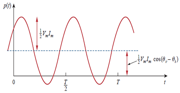
Since \(p(t)\) varies rapidly and is hard to measure, the useful quantity is its average over one period:
Splitting the integral into the two terms: the first integrand is constant and integrates to itself; the second is a sinusoid whose average over a whole number of periods is exactly zero. Hence
In phasor terms, with \(\mathbf{V} = V_{m}\angle\theta_{v}\) and \(\mathbf{I} = I_{m}\angle\theta_{i}\), note that
so the average power is simply the real part:
Note the conjugate. Using \(\mathbf{V}\mathbf{I}\) rather than \(\mathbf{V}\mathbf{I}^{*}\) would give the wrong angle and hence the wrong power — a mistake worth guarding against.
Purely resistive load. Here \(\theta_{v} = \theta_{i}\), so \(\cos 0 = 1\) and
Purely reactive load. Here \(\theta_{v}-\theta_{i} = \pm90^{\circ}\), so
This is the central result of the chapter, and it deserves to be stated plainly: a resistive load absorbs power at all times, while a purely reactive load — an ideal inductor or capacitor — absorbs zero average power. Energy flows in for a quarter-cycle and back out during the next, indefinitely, with nothing consumed.
Problem. Given \(v(t) = 120\cos\left(377t + 45^{\circ}\right)~\mathrm{V}\) and \(i(t) = 10\cos\left(377t - 10^{\circ}\right)~\mathrm{A}\), find the instantaneous power and the average power absorbed.
Solution. The product is
Applying the product identity:
The constant part is the average power, which the general formula confirms:
Note the doubled frequency: the source runs at 377 rad/s but the power oscillates at 754 rad/s. Note too that the oscillating amplitude of 600 W exceeds the average of 344.2 W, so \(p(t)\) goes negative for part of each cycle — energy really does flow back to the source.
Maximum Average Power Transfer
Section 4.8 showed that a DC source delivers maximum power when \(R_{L} = R_{Th}\). The AC case has an extra degree of freedom, because both the source and the load now have reactance as well as resistance.
With \(\mathbf{Z}_{Th} = R_{Th}+jX_{Th}\) and \(\mathbf{Z}_{L} = R_{L}+jX_{L}\), the current and the power delivered are
This must be maximised with respect to two variables. Setting \(\partial P/\partial X_{L} = 0\) requires the term \(\left(X_{Th}+X_{L}\right)\) to vanish — which makes sense, since that term appears only in the denominator and any non-zero value can only reduce \(P\):
Setting \(\partial P/\partial R_{L} = 0\) then gives
once the first condition is imposed. Combining the two:
Maximum average power is transferred when the load impedance is the complex conjugate of the Thévenin impedance. This is the conjugate match, and it is not the same as \(\mathbf{Z}_{L} = \mathbf{Z}_{Th}\) — a distinction that catches many students.
Physically, the conjugate cancels the source reactance: \(X_{Th}+X_{L} = 0\) makes the total circuit purely resistive, which is resonance. With the reactance gone, the remaining problem is the DC one of Chapter 4, and its answer is \(R_{L}=R_{Th}\) as before. Substituting back:
The factor of 8 rather than the DC formula's 4 arises because \(\left|\mathbf{V}_{Th}\right|\) here is an amplitude, not an RMS value. In terms of RMS quantities the formula reverts to \(V_{Th,\mathrm{rms}}^{2}/4R_{Th}\).
A restricted case. If the load is constrained to be purely resistive — no reactance available — then \(X_{L}=0\) and the optimum becomes
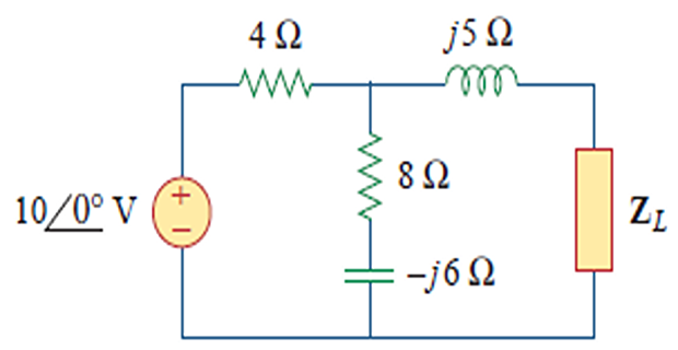
Problem. A network consists of a \(10\angle 0^{\circ}~\mathrm{V}\) source feeding a 4 \(\Omega\) resistor, with an \(\left(8-j6\right)~\Omega\) branch in parallel, and a \(j5~\Omega\) inductor in series with the output terminals. Determine the \(\mathbf{Z}_{L}\) that maximises the average power drawn, and find \(P_{\max}\).
Solution. First the Thévenin equivalent:
The optimum load is the conjugate:
and the maximum power follows:
Note that the load must be capacitive (\(-j4.467\)) even though the source is inductive. The load reactance exists precisely to cancel the source reactance, and it must therefore be of opposite sign.
Effective or RMS Values
A sinusoid's average value over a full cycle is zero, so quoting it is useless. The meaningful measure of a periodic waveform's "size" is defined by what it does:
The effective value of a periodic current is the DC current that delivers the same average power to a resistor.
Equating the average power of the periodic current with that of the equivalent DC:
The name follows the operations performed, read inside out: take the root of the mean of the square. The effective value and the RMS value are the same thing, and the terms are used interchangeably.
For a sinusoid \(i = I_{m}\cos\omega t\), using \(\cos^{2}\theta = \tfrac{1}{2}\left(1+\cos 2\theta\right)\):
This factor applies to sinusoids only. Any other waveform has its own ratio, and using \(1/\sqrt{2}\) indiscriminately is a common and serious error.
Average power written in RMS terms loses the awkward factor of one half:
This is why power engineering works almost entirely in RMS. When a supply is described as "240 V", that is an RMS value: the peak is \(240\sqrt{2} = 339~\mathrm{V}\), which is what the insulation must withstand.
Two dimensionless ratios characterise a waveform's shape independently of its size:
where \(V_{\mathrm{av}}\) is the average taken over a half-cycle for a symmetrical waveform. For a sinusoid, \(V_{\mathrm{av}} = 2V_{m}/\pi = 0.6366V_{m}\), giving
The peak factor matters practically. A rectifier-fed load draws a current whose peak factor is far higher than 1.414, so a cable rated by RMS current may still see peaks that saturate a transformer or trip a breaker.
| Waveform | \(V_{\mathrm{rms}}\) | Form factor | Peak factor |
|---|---|---|---|
| Sinusoid | \(V_{m}/\sqrt{2} = 0.7071V_{m}\) | 1.111 | 1.414 |
| Half-wave rectified sine | \(V_{m}/2 = 0.5V_{m}\) | 1.571 | 2.000 |
| Full-wave rectified sine | \(0.7071V_{m}\) | 1.111 | 1.414 |
| Square wave | \(V_{m}\) | 1.000 | 1.000 |
| Triangular / sawtooth | \(V_{m}/\sqrt{3} = 0.5774V_{m}\) | 1.155 | 1.732 |
Problem. A periodic current rises linearly as \(i = 4t~\mathrm{A}\) over \(0 < t < 2~\mathrm{s}\) and then repeats with period \(T = 2~\mathrm{s}\). Find its RMS value, its peak factor, and the average power it delivers to a 5 \(\Omega\) resistor.
Solution. Apply the definition directly:
The peak value is \(4(2) = 8~\mathrm{A}\), so
which matches the sawtooth entry in the table above. The average power delivered is
The point of this example is that \(I_{m}/\sqrt{2} = 8/1.414 = 5.657~\mathrm{A}\) would have been badly wrong — 22 % too high in current, and since power goes as the square, 50 % too high in power (160 W instead of 106.7 W). The \(1/\sqrt{2}\) factor is a property of the sinusoid, not of periodic waveforms in general.
Apparent Power and Power Factor
Writing the average power as
separates it into two factors, and each deserves a name.
Apparent power \(S = V_{\mathrm{rms}}I_{\mathrm{rms}}\) is what the power appears to be from a casual multiplication of the meter readings. Its unit is the volt-ampere (VA), deliberately distinct from the watt as a reminder that it is not power in the energetic sense.
Power factor \(\mathrm{pf} = \cos\left(\theta_{v}-\theta_{i}\right) = P/S\) is the dimensionless fraction of apparent power that does useful work. It lies between 0 and 1.
The angle \(\theta_{v}-\theta_{i}\) is called the power factor angle, and it equals the angle of the load impedance, since
Because the cosine is an even function, the power factor alone does not reveal the sign of the angle. The qualifier must always be given:
Lagging power factor — current lags voltage, \(\theta_{v}-\theta_{i} > 0\), inductive load. Nearly all industrial loads.
Leading power factor — current leads voltage, \(\theta_{v}-\theta_{i} < 0\), capacitive load.
Unity power factor — in phase, purely resistive.
"A power factor of 0.8" is an incomplete specification; "0.8 lagging" is a complete one.

Complex Power
All the quantities so far can be packed into a single complex number. Define the complex power as
Expanding it in polar and then rectangular form:
Substituting \(\mathbf{V}_{\mathrm{rms}} = \mathbf{Z}\mathbf{I}_{\mathrm{rms}}\) gives an equally useful form:
so the real part of the complex power comes from the resistance and the imaginary part from the reactance — precisely as one would hope.
| Quantity | Symbol | Definition | Unit |
|---|---|---|---|
| Complex power | \(\mathbf{S}\) | \(\mathbf{V}_{\mathrm{rms}}\mathbf{I}_{\mathrm{rms}}^{*} = P+jQ\) | VA |
| Apparent power | \(S\) | \(\left|\mathbf{S}\right| = \sqrt{P^{2}+Q^{2}}\) | VA |
| Real (average) power | \(P\) | \(\mathrm{Re}\left(\mathbf{S}\right) = S\cos\theta\) | W |
| Reactive power | \(Q\) | \(\mathrm{Im}\left(\mathbf{S}\right) = S\sin\theta\) | VAR |
| Power factor | pf | \(P/S = \cos\theta\) | — |
Real power \(P\) is the average power in watts actually delivered to and dissipated by the load. It is the only useful power, and the only quantity an energy meter records.
Reactive power \(Q\) measures the energy exchanged back and forth between the source and the reactive part of the load. Its unit is the volt-ampere reactive (VAR) — again deliberately distinct from the watt. Its sign classifies the load:
\(Q = 0\) for a resistive load — unity power factor.
\(Q > 0\) for an inductive load — lagging power factor. An inductor is said to absorb reactive power.
\(Q < 0\) for a capacitive load — leading power factor. A capacitor supplies reactive power.
That last pair of statements is the entire basis of power factor correction: if an inductive load absorbs VARs and a capacitor supplies them, then putting a capacitor next to the load lets them settle the account locally instead of dragging it back to the generator.
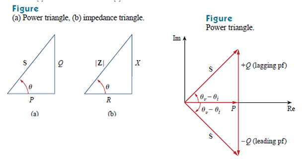
Since \(\mathbf{S} = P + jQ\) is a complex number, it can be drawn in the complex plane as a right triangle with \(P\) horizontal, \(Q\) vertical, and \(S\) as the hypotenuse.
The triangle encodes every relationship at a glance:
Note the analogy with the impedance triangle of Section 9.7: both have the same angle \(\theta\), because \(\mathbf{S} = I_{\mathrm{rms}}^{2}\mathbf{Z}\) and multiplying by a positive real number does not change an angle.
Problem. The voltage across a load is \(v(t) = 60\cos\left(\omega t - 10^{\circ}\right)~\mathrm{V}\) and the current through it, in the direction of the voltage drop, is \(i(t) = 1.5\cos\left(\omega t + 50^{\circ}\right)~\mathrm{A}\). Find (a) the complex and apparent powers, (b) the real and reactive powers, (c) the power factor and the load impedance.
Solution. Convert to RMS phasors:
(a) The complex power uses the conjugate of the current:
(b) In rectangular form:
(c) The power factor and impedance:
Every indicator agrees that the load is capacitive: the negative \(Q\), the leading power factor, the negative impedance angle and the negative reactance. Note that the load draws 45 VA from the supply while consuming only 22.5 W — exactly half the apparent power is doing no useful work.
Conservation of AC Power
Section 1.5 established that power is conserved in a DC circuit. The same holds in AC, and it holds separately for the real and reactive parts:
The complex powers of the individual elements add to the complex power supplied by the source, whether the elements are in series or in parallel. This follows from the linearity of the phasor transform and is a direct consequence of Kirchhoff's laws.
What does not add is apparent power. Since \(S = \left|\mathbf{S}\right|\) is a magnitude, and magnitudes of complex numbers do not add, \(S_{\text{total}} \neq \sum S_{k}\) in general. This is exactly the trap of Section 9.9, in a new guise.
Conservation of complex power is the best available check on an AC circuit solution. Compute \(\mathbf{S}\) for every element, add them, and confirm the sum matches the source. It costs a minute and catches most errors.
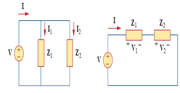
Problem. A \(220\angle 0^{\circ}~\mathrm{V}\) rms source feeds a load of \(\left(15-j10\right)~\Omega\) through a transmission line of impedance \(\left(4+j2\right)~\Omega\). Find the complex power supplied by the source and absorbed by the load, and verify conservation.
Solution. The total impedance and the line current:
The source complex power:
so the source supplies 2163.8 W of real power and the circuit is net capacitive, returning 911.1 VAR.
For the load, the voltage across it is
The line absorbs the remainder, and being purely a series impedance its complex power is \(\left|\mathbf{I}\right|^{2}\mathbf{Z}_{\text{line}}\):
Check:
Both the real and the reactive parts balance exactly. Observe also that the apparent powers do not: \(2053.0 + 509.3 = 2562.3 \neq 2347.7\) VA. Only the complex powers add.
Power Factor Correction
Nearly every practical load is inductive. Induction motors, transformers, fluorescent ballasts, welding sets, washing machines, air conditioners and refrigerators all operate at a lagging power factor, often as low as 0.6 or 0.7.
The consequences fall on the supply system rather than the consumer's energy meter. For a given real power \(P\) at a fixed voltage, the current drawn is
so halving the power factor doubles the current. That extra current dissipates \(I^{2}R\) in every cable and transformer between the load and the generator, and it consumes capacity that could have carried useful load. None of it registers on an energy meter.
Power factor correction is the process of increasing the power factor without altering the voltage or current supplied to the original load. The inductive nature of the load cannot be changed — but a capacitor connected in parallel with it can supply the reactive power that the load demands, so that the supply need not.
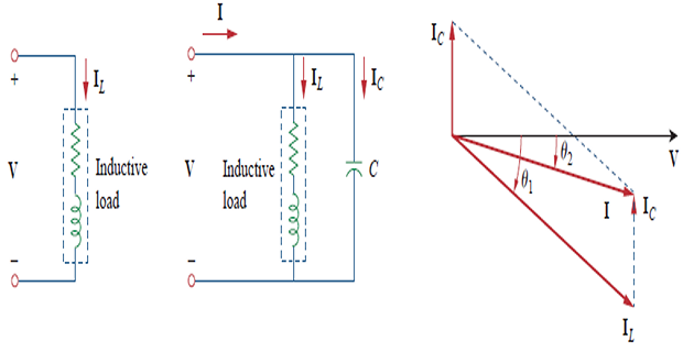
Design. The real power is unchanged by the capacitor, since an ideal capacitor consumes none. Only the reactive power changes:
The capacitor must supply the difference:
and since a capacitor across the supply voltage provides \(Q_{C} = V_{\mathrm{rms}}^{2}/X_{C} = \omega C V_{\mathrm{rms}}^{2}\),
The capacitor is connected in parallel with the load, not in series, so that the load continues to see the same voltage and behaves exactly as before. From the supply's point of view the two together draw less current at a better angle.
Problem. A load draws 4 kW at a power factor of 0.8 lagging from a 240 V rms, 50 Hz supply. Find the capacitance required to raise the power factor to 0.95 lagging, and the reduction in supply current achieved.
Solution. The two phase angles:
The reactive powers before and after:
and hence the capacitance, with \(\omega = 2\pi(50) = 314.2~\mathrm{rad/s}\):
The benefit. The supply current before and after:
A 16 % reduction in current means a 29 % reduction in \(I^{2}R\) losses in the supply cable, for the cost of one capacitor. The load itself is entirely unaffected — it still draws its 4 kW at 0.8 pf. What has changed is that the reactive current now circulates locally between load and capacitor instead of travelling back to the generator.
Why not correct to unity? Two reasons. The capacitance needed rises steeply as unity is approached — going from 0.95 to 1.0 would need almost as much again — and an overcorrected system becomes leading, which brings its own problems including possible resonance with the supply inductance. Utilities typically require 0.9 to 0.95, not 1.0.
Power Measurement
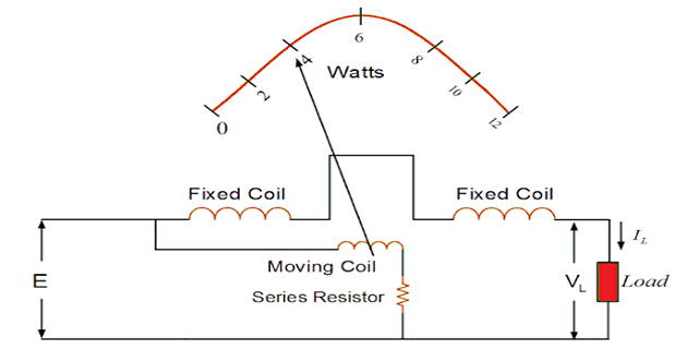
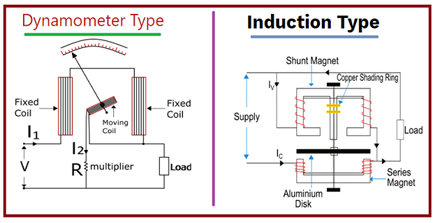
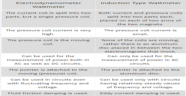
A wattmeter measures average power, and it must therefore respond to the product of instantaneous voltage and current rather than to either alone. The classical instrument that achieves this is the electrodynamometer.
It contains two coils. The current coil is of few turns and low resistance, connected in series with the load so that it carries the load current. The voltage coil — or pressure coil — is of many turns with a high series resistance, connected across the load so that its current is proportional to the load voltage. The deflecting torque is proportional to the product of the two coil currents, and because the moving system has too much inertia to follow a \(2\omega\) variation, the pointer settles at the average of that product:
The instrument reads watts directly, and — unlike a moving-iron or moving-coil meter — it reads correctly on both AC and DC.
Low power factor wattmeters. At very low power factor the deflecting torque becomes small, and a standard instrument would give an unreadably small deflection with poor accuracy. An LPF wattmeter uses a voltage coil of fewer turns and compensating windings to restore usable deflection. Its scale is then calibrated for a nominal power factor, and the true power requires a multiplying factor:
Forgetting the multiplying factor is a classical laboratory error, and it produces a result wrong by a factor of several.
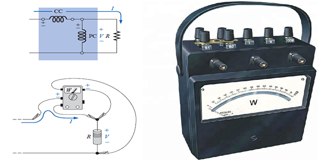
Chapter 12 returns to power measurement for three-phase systems, where the two-wattmeter method allows the total power of a three-wire system to be measured with only two instruments — and, remarkably, allows the power factor to be deduced from their two readings.
Applications: The Cost of Electricity
Section 1.7 computed a domestic bill from energy alone. Industrial tariffs are different, and the difference is where the economics of power factor becomes concrete.
A domestic consumer pays only for energy, in kWh — a real-power quantity. Power factor is irrelevant to the bill, which is why domestic appliances are not required to correct it.
An industrial consumer typically pays two charges:
an energy charge per kWh, exactly as domestic; plus
a demand charge per kVA of maximum demand — an apparent-power quantity, which depends directly on power factor.
The demand charge exists because the utility must size its cables, transformers and switchgear for the current the consumer draws, and that current is set by kVA rather than kW. A consumer at poor power factor demands more of the network's capacity while paying the same energy charge, and the demand charge recovers that cost. Many tariffs go further and impose an explicit penalty below a threshold power factor, or a rebate above it.
Problem. A factory draws 500 kW at a power factor of 0.75 lagging. The tariff includes a demand charge of ₹300 per kVA of maximum demand per month. Find the monthly saving if the power factor is corrected to 0.95.
Solution. The apparent power before and after:
The demand charges:
Over ₹500,000 per year, for a bank of capacitors that would pay for itself within months. The energy charge does not change at all — the factory still consumes 500 kW of real power and its energy meter registers exactly the same kWh. The entire saving comes from the reduced apparent power, and that is why power factor correction is a standard part of any industrial installation.
There is a second, less visible saving: the reduced current also cuts \(I^{2}R\) losses in the factory's own distribution, and releases transformer capacity that would otherwise have to be bought as new plant.
Summary and Key Formulas
Instantaneous power has a constant part and a part oscillating at \(2\omega\) whose average is zero.
Average power is \(P = \tfrac{1}{2}V_{m}I_{m}\cos(\theta_{v}-\theta_{i}) = \tfrac{1}{2}\mathrm{Re}\left[\mathbf{V}\mathbf{I}^{*}\right]\). A purely reactive element absorbs none.
Maximum average power transfer requires the conjugate match \(\mathbf{Z}_{L} = \mathbf{Z}_{Th}^{*}\), giving \(P_{\max} = \left|\mathbf{V}_{Th}\right|^{2}/8R_{Th}\).
The RMS value is the DC equivalent for power delivery. For a sinusoid it is \(V_{m}/\sqrt{2}\), but that factor applies to sinusoids only.
Apparent power \(S = V_{\mathrm{rms}}I_{\mathrm{rms}}\) in VA; power factor \(\mathrm{pf} = P/S = \cos\theta\), always qualified as leading or lagging.
Complex power \(\mathbf{S} = \mathbf{V}_{\mathrm{rms}}\mathbf{I}_{\mathrm{rms}}^{*} = P + jQ\), with \(Q>0\) inductive and \(Q<0\) capacitive.
Complex power is conserved, so \(P\) and \(Q\) each add separately — but apparent power does not add.
Power factor correction uses a shunt capacitor supplying \(Q_{C} = P\left(\tan\theta_{1}-\tan\theta_{2}\right)\).
A wattmeter reads average power; industrial tariffs charge for kVA demand, which is what makes correction economic.
| Result | Formula | Notes |
|---|---|---|
| Instantaneous power | \(p = \tfrac{1}{2}V_mI_m\cos\theta + \tfrac{1}{2}V_mI_m\cos\left(2\omega t+\theta_v+\theta_i\right)\) | second term at \(2\omega\) |
| Average power | \(P = \tfrac{1}{2}V_mI_m\cos\left(\theta_v-\theta_i\right)\) | amplitudes |
| Average power, phasors | \(P = \tfrac{1}{2}\mathrm{Re}\left[\mathbf{V}\mathbf{I}^{*}\right]\) | note the conjugate |
| Reactive element | \(P = 0\) | \(\cos 90^{\circ} = 0\) |
| Conjugate match | \(\mathbf{Z}_L = \mathbf{Z}_{Th}^{*}\) | not \(\mathbf{Z}_{Th}\) |
| Maximum power | \(P_{\max} = \dfrac{\left|\mathbf{V}_{Th}\right|^{2}}{8R_{Th}}\) | amplitude; use \(4R_{Th}\) for rms |
| Resistive load only | \(R_L = \left|\mathbf{Z}_{Th}\right|\) | when \(X_L\) unavailable |
| RMS definition | \(X_{\mathrm{rms}} = \sqrt{\dfrac{1}{T}\displaystyle\int_{0}^{T}x^{2}dt}\) | any periodic waveform |
| RMS of a sinusoid | \(V_{\mathrm{rms}} = V_m/\sqrt{2}\) | sinusoids only |
| Form factor | \(V_{\mathrm{rms}}/V_{\mathrm{av}}\) | 1.111 for a sinusoid |
| Peak factor | \(V_m/V_{\mathrm{rms}}\) | 1.414 for a sinusoid |
| Average power, rms | \(P = V_{\mathrm{rms}}I_{\mathrm{rms}}\cos\theta = I_{\mathrm{rms}}^{2}R\) | no factor of one half |
| Apparent power | \(S = V_{\mathrm{rms}}I_{\mathrm{rms}} = \left|\mathbf{S}\right|\) | volt-amperes |
| Power factor | \(\mathrm{pf} = P/S = \cos\left(\theta_v-\theta_i\right)\) | state leading or lagging |
| Complex power | \(\mathbf{S} = \mathbf{V}_{\mathrm{rms}}\mathbf{I}_{\mathrm{rms}}^{*} = P+jQ\) | also \(I_{\mathrm{rms}}^{2}\mathbf{Z}\) |
| Power triangle | \(S^{2} = P^{2}+Q^{2}\), \(Q = P\tan\theta\) | same angle as \(\mathbf{Z}\) |
| Conservation | \(\mathbf{S} = \sum\mathbf{S}_k\) | \(P\) and \(Q\) add; \(S\) does not |
| Correction capacitor | \(C = \dfrac{P\left(\tan\theta_1-\tan\theta_2\right)}{\omega V_{\mathrm{rms}}^{2}}\) | connected in parallel |
| Supply current | \(I_{\mathrm{rms}} = \dfrac{P}{V_{\mathrm{rms}}\,\mathrm{pf}}\) | inverse in pf |
Common Mistakes
Omitting the conjugate in \(\mathbf{V}\mathbf{I}^{*}\). Using \(\mathbf{V}\mathbf{I}\) gives the angle \(\theta_{v}+\theta_{i}\) instead of the difference, and hence the wrong \(P\) and \(Q\) entirely.
Mixing amplitude and RMS forms. \(P = \tfrac{1}{2}V_{m}I_{m}\cos\theta\) uses amplitudes; \(P = V_{\mathrm{rms}}I_{\mathrm{rms}}\cos\theta\) does not have the half. Using both halves, or neither, gives an error of a factor of two.
Applying \(V_{m}/\sqrt{2}\) to a non-sinusoidal waveform. That ratio belongs to the sinusoid alone. Use the integral definition for anything else.
Writing \(\mathbf{Z}_{L} = \mathbf{Z}_{Th}\) for maximum power transfer. The AC condition is the conjugate. The load reactance must be opposite in sign to the source reactance.
Adding apparent powers. \(S\) is a magnitude and magnitudes do not add. Add the complex powers and take the magnitude at the end.
Quoting a power factor without "leading" or "lagging". The cosine is even, so 0.8 alone does not determine the angle's sign.
Confusing the units. Watts for \(P\), VAR for \(Q\), VA for \(S\). They are numerically different quantities and the distinct units exist to prevent exactly this error.
Connecting the correction capacitor in series. It goes in parallel, so the load continues to see its rated voltage.
Assuming correction reduces the energy bill. It reduces the demand charge and the distribution losses. The kWh consumed by the load is unchanged.
Forgetting a wattmeter's multiplying factor on a low-power-factor instrument. The scale reading is not the answer.
Chapter Review
Work these before opening the answers. State units precisely — W, VAR or VA — and qualify every power factor.
P11.1 A load has \(v = 160\cos\left(\omega t + 20^{\circ}\right)~\mathrm{V}\) and \(i = 4\cos\left(\omega t - 40^{\circ}\right)~\mathrm{A}\). Find the average power.
Show answer
\[P = \tfrac{1}{2}\left(160\right)\left(4\right)\cos\left(20^{\circ}+40^{\circ}\right) = 320\cos 60^{\circ} = 160.0~\mathrm{W}\]P11.2 Find the RMS value of a square wave that alternates between \(+6~\mathrm{A}\) and \(-6~\mathrm{A}\), and its peak factor.
Show answer
The square of the waveform is 36 at all times, so its mean is 36 andA square wave is the only common waveform whose RMS equals its peak.\[I_{\mathrm{rms}} = \sqrt{36} = 6.000~\mathrm{A}, \qquad \text{peak factor} = \frac{6}{6} = 1.000\]P11.3 A network has \(\mathbf{Z}_{Th} = \left(6+j8\right)~\Omega\) and \(\mathbf{V}_{Th} = 40\angle 0^{\circ}~\mathrm{V}\) (amplitude). Find \(\mathbf{Z}_{L}\) for maximum power transfer and the value of \(P_{\max}\).
Show answer
\[\mathbf{Z}_{L} = \mathbf{Z}_{Th}^{*} = \left(6-j8\right)~\Omega\]\[P_{\max} = \frac{40^{2}}{8\left(6\right)} = \frac{1600}{48} = 33.33~\mathrm{W}\]P11.4 For the same network, what purely resistive load gives maximum power, and how much?
Show answer
\[R_{L} = \left|\mathbf{Z}_{Th}\right| = \sqrt{36+64} = 10~\Omega\]\[\left|\mathbf{I}\right| = \frac{40}{\left|6+j8+10\right|} = \frac{40}{\left|16+j8\right|} = \frac{40}{17.89} = 2.236~\mathrm{A}\]Less than the 33.33 W of the conjugate match, as expected.\[P = \tfrac{1}{2}\left(2.236\right)^{2}\left(10\right) = 25.00~\mathrm{W}\]P11.5 A load draws \(\mathbf{S} = \left(1200 + j1600\right)~\mathrm{VA}\). Find \(S\), the power factor, and state whether the load is inductive or capacitive.
Show answer
Since \(Q > 0\) the load is inductive.\[S = \sqrt{1200^{2}+1600^{2}} = 2000~\mathrm{VA}, \qquad \mathrm{pf} = \frac{1200}{2000} = 0.6000\ \text{lagging}\]P11.6 A 230 V rms, 50 Hz supply feeds a 3 kW load at 0.7 pf lagging. Find the supply current, and the current after correction to 0.9 lagging.
Show answer
A reduction of 22.22 %.\[I_{1} = \frac{3000}{\left(230\right)\left(0.7\right)} = 18.63~\mathrm{A}, \qquad I_{2} = \frac{3000}{\left(230\right)\left(0.9\right)} = 14.49~\mathrm{A}\]P11.7 Find the capacitance required in P11.6.
Show answer
\[\theta_{1} = \cos^{-1}0.7 = 45.57^{\circ}, \quad \tan\theta_{1} = 1.0202; \qquad \theta_{2} = \cos^{-1}0.9 = 25.84^{\circ}, \quad \tan\theta_{2} = 0.4843\]\[Q_{C} = 3000\left(1.0202 - 0.4843\right) = 1607.7~\mathrm{VAR}\]\[C = \frac{1607.7}{\left(314.2\right)\left(230\right)^{2}} = 96.72~\mu\mathrm{F}\]P11.8 A source supplies \(\left(800+j600\right)~\mathrm{VA}\). One load absorbs \(\left(500+j400\right)~\mathrm{VA}\). Find the complex power of the second load, and check that apparent powers do not add.
Show answer
Apparent powers: \(\left|\mathbf{S}_{s}\right| = 1000\), \(\left|\mathbf{S}_{1}\right| = 640.3\), \(\left|\mathbf{S}_{2}\right| = 360.6\). Since \(640.3+360.6 = 1000.9 \neq 1000\), the apparent powers indeed do not add — though they come close here because both loads have similar angles.\[\mathbf{S}_{2} = \left(800+j600\right)-\left(500+j400\right) = \left(300+j200\right)~\mathrm{VA}\]P11.9 A factory draws 800 kW at 0.7 pf. At ₹250 per kVA of demand, what is the monthly saving if corrected to 0.92?
Show answer
\[S_{1} = \frac{800}{0.7} = 1142.9~\mathrm{kVA}, \qquad S_{2} = \frac{800}{0.92} = 869.6~\mathrm{kVA}\]\[\text{Saving} = \left(1142.9-869.6\right)\left(250\right) = \text{Rs.}\,68\,320\ \text{per month}\]P11.10 An inductor of reactance \(j20~\Omega\) carries 5 A rms. Find its real and reactive power.
Show answer
So \(P = 0~\mathrm{W}\) and \(Q = 500~\mathrm{VAR}\). The inductor consumes no energy yet demands 500 VAR from the supply — the central paradox of this chapter, in one line.\[\mathbf{S} = I_{\mathrm{rms}}^{2}\mathbf{Z} = \left(25\right)\left(j20\right) = j500~\mathrm{VA}\]
MCQ 1. The instantaneous power in an AC circuit oscillates at a frequency of:
(a) \(\omega\) (b) \(2\omega\) (c) \(\omega/2\) (d) it is constantShow answer
(b) \(2\omega\), from the product identity. The average part is constant.MCQ 2. The average power absorbed by an ideal inductor is:
(a) \(\tfrac{1}{2}V_mI_m\) (b) \(V_{\mathrm{rms}}I_{\mathrm{rms}}\) (c) zero (d) infiniteShow answer
(c) zero, since \(\cos 90^{\circ} = 0\). It still draws current and reactive power.MCQ 3. The unit of reactive power is the:
(a) watt (b) volt-ampere (c) VAR (d) jouleShow answer
(c) VAR. Watts are for \(P\) and volt-amperes for \(S\).MCQ 4. For maximum average power transfer in an AC circuit:
(a) \(\mathbf{Z}_L = \mathbf{Z}_{Th}\) (b) \(\mathbf{Z}_L = \mathbf{Z}_{Th}^{*}\) (c) \(R_L = R_{Th}\) only (d) \(\mathbf{Z}_L = 0\)Show answer
(b) the conjugate. Option (a) is the frequent error — it would double the reactance rather than cancelling it.MCQ 5. The RMS value of a square wave of amplitude \(V_m\) is:
(a) \(V_m/\sqrt{2}\) (b) \(V_m/2\) (c) \(V_m\) (d) \(V_m/\sqrt{3}\)Show answer
(c) \(V_m\). The square of the waveform is constant, so its mean equals \(V_m^{2}\). Option (a) applies only to sinusoids.MCQ 6. A load with \(Q < 0\) is:
(a) inductive (b) capacitive (c) resistive (d) at unity pfShow answer
(b) capacitive, with a leading power factor. A capacitor supplies reactive power.MCQ 7. A load absorbing 800 W at 0.8 pf has an apparent power of:
(a) 640 VA (b) 800 VA (c) 1000 VA (d) 1250 VAShow answer
(c) 1000 VA. \(S = P/\mathrm{pf} = 800/0.8\). Option (a) multiplies instead of dividing.MCQ 8. In a circuit with several loads, the quantity that does not add is:
(a) real power (b) reactive power (c) complex power (d) apparent powerShow answer
(d) apparent power, being a magnitude. The other three all add.MCQ 9. A shunt capacitor for power factor correction is connected:
(a) in series with the load (b) in parallel with the load (c) in series with the supply (d) across the source onlyShow answer
(b) in parallel, so that the load continues to receive its rated voltage.MCQ 10. Power factor correction reduces:
(a) the kWh consumed (b) the real power (c) the supply current (d) the load voltageShow answer
(c) the supply current — and hence the kVA demand and the distribution losses. The kWh and the real power are unchanged.
An ideal inductor consumes no energy, yet it is described as "absorbing reactive power". Explain what is actually being demanded of the supply, and why it costs the utility money.
Reactive power has its own unit, the VAR, distinct from the watt even though both are dimensionally volt-amperes. Argue for and against this convention.
Why does maximum power transfer in AC require the conjugate rather than the equal impedance? Give both an algebraic and a physical explanation.
The RMS value is defined by equal power delivery to a resistor. Why is this a better definition of "size" than the peak value or the average of the magnitude?
Power factor correction reduces the current without altering the load. Where does the reactive current go after correction, and what does this imply about where the capacitor should be installed?
Utilities generally require a power factor of 0.9 to 0.95 rather than 1.0. Give two independent reasons why perfect correction is not the target.
Everything in this chapter has concerned a single-phase supply — one source, one pair of conductors. Almost all electrical energy is generated, transmitted and consumed in three-phase form instead, and Chapter 12 explains why.
Three sources of equal magnitude, displaced by 120°, produce something remarkable: the total instantaneous power delivered to a balanced load is constant, with no \(2\omega\) ripple at all. A three-phase motor therefore produces steady torque where a single-phase one pulsates. Three-phase transmission also carries more power per kilogram of conductor, and generates the rotating magnetic field on which the induction motor depends.
All the machinery of this chapter carries forward — complex power, power factor, correction — applied now to three phases at once. Chapter 12 also returns to power measurement with the two-wattmeter method, which measures three-phase power with two instruments and reveals the power factor from their ratio.