- Determine the initial values \(x(0^{+})\) and \(dx(0^{+})/dt\) together with the final value \(x(\infty)\).
- Derive the second-order differential equation and its characteristic equation for series and parallel RLC circuits.
- Compute the neper frequency \(\alpha\) and the resonant frequency \(\omega_{0}\), and form the damping ratio.
- Classify a response as overdamped, critically damped or underdamped, and write the appropriate form.
- Evaluate the arbitrary constants from the two initial conditions.
- Find the complete step response as forced plus natural parts.
- Analyse a general second-order circuit that is neither purely series nor purely parallel.
- Construct the dual of a planar network and use duality to halve the work.
- Explain how an RLC transient produces the high voltage in an automobile ignition system.
Introduction
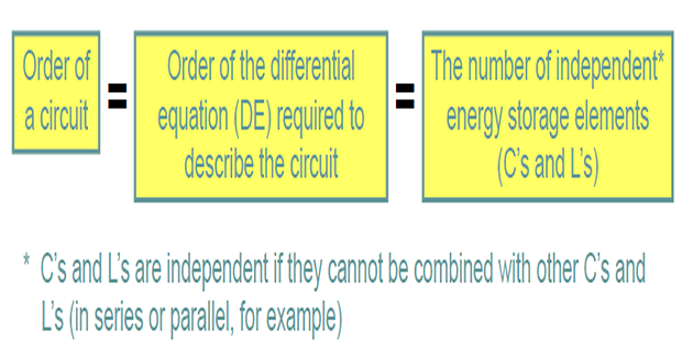
Chapter 7 dealt with circuits containing a single storage element, whose response was always a simple exponential — monotonic, decaying, never overshooting. A second-order circuit contains two irreducible storage elements, and applying Kirchhoff's laws to it produces a second-order differential equation.
The extra element changes the behaviour qualitatively, not merely quantitatively. With a capacitor and an inductor in the same circuit, energy need not simply drain into the resistors: it can be handed back and forth between the capacitor's electric field and the inductor's magnetic field, passing through the resistance a little at a time. When that exchange dominates, the response oscillates before settling — the circuit rings.
Whether it rings, and how much, depends on a single competition: dissipation in the resistance against exchange between the two storage elements. Quantifying that competition, and reading off the three qualitatively different outcomes it produces, is what this chapter is about.
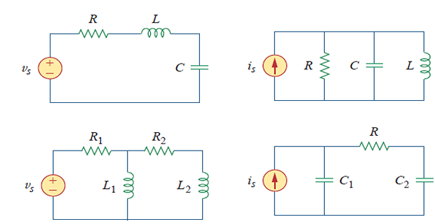
The word irreducible matters. Two capacitors that can be combined into one by the rules of Section 6.4 give a first-order circuit, not a second-order one. What is required is a capacitor and an inductor, or two storage elements that cannot be merged.
Finding Initial and Final Values
A second-order equation needs two initial conditions, not one. This is the single greatest source of difficulty in the chapter, and it is worth confronting before any differential equation appears.
Throughout this chapter, unless stated otherwise, \(v\) denotes capacitor voltage and \(i\) denotes inductor current — the two continuous variables. The quantities normally required are
The two continuity conditions remain the foundation, exactly as in Chapter 7:
Take care with polarity: apply the passive sign convention consistently to the capacitor voltage and the inductor current, and do not change the reference direction halfway through a problem.
The derivative conditions are the new work, and they come from the element relations of Chapter 6 read backwards:
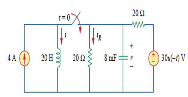
In words: to find the initial rate of change of capacitor voltage, find the initial capacitor current; to find the initial rate of change of inductor current, find the initial inductor voltage. Both of those are obtained by analysing the circuit at \(t = 0^{+}\) with the now-known values of \(v(0^{+})\) and \(i(0^{+})\) treated as a fixed voltage source and a fixed current source respectively.
Final values are easier: at \(t = \infty\) the circuit is in DC steady state again, so the capacitor becomes an open circuit and the inductor a short circuit, exactly as in Section 6.8.
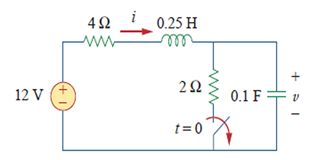
Problem. A 12 V source drives a 4 \(\Omega\) resistor in series with an inductor \(L = 0.25~\mathrm{H}\), followed by a capacitor \(C = 0.1~\mathrm{F}\) which has a 2 \(\Omega\) resistor across it. A switch across the 2 \(\Omega\) branch has been closed a long time and opens at \(t = 0\). Find (a) \(i(0^{+})\) and \(v(0^{+})\), (b) \(di(0^{+})/dt\) and \(dv(0^{+})/dt\), (c) \(i(\infty)\) and \(v(\infty)\).
(a) The instant before, and the instant after. For \(t < 0\) the circuit has settled, so the inductor is a short and the capacitor an open circuit. The current flows through the 4 \(\Omega\) and 2 \(\Omega\) in series:
By continuity these values carry across the switching instant:
(b) The derivatives. At \(t = 0^{+}\) the switch has opened, so the whole inductor current is forced into the capacitor:
For the other derivative, apply KVL around the loop at \(t = 0^{+}\) using the known values:
(c) The final values. After a long time the circuit settles again: the capacitor is an open circuit, so no current can flow at all, and the full source voltage appears across it.
Note that \(di(0^{+})/dt = 0\) does not mean the current stays at 2 A. It means the current is momentarily at a turning point — its second derivative is what carries it onward. Reading too much into a zero first derivative is a classic misstep.
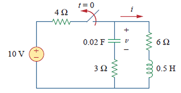
The Source-Free Series RLC Circuit
Consider a series loop of \(R\), \(L\) and \(C\) with no source, in which the capacitor is initially charged to \(V_{0}\) and the inductor carries an initial current \(I_{0}\).
Derivation. Applying KVL around the loop, with the capacitor voltage written as an integral of the current:
The integral is awkward, so differentiate the whole equation with respect to time and divide by \(L\):
A second-order homogeneous differential equation with constant coefficients. Its solution is assumed exponential, \(i = A e^{st}\), and substituting gives
Neither \(A\) nor \(e^{st}\) can vanish if a solution is to exist, so the bracket must be zero. This is the characteristic equation:
Solving by the quadratic formula gives the two natural frequencies:
The result becomes far clearer with two definitions:
and the characteristic equation takes the standard form used throughout engineering:
\(\alpha\) is the neper frequency or damping factor, in nepers per second. It measures how fast the response dies away, and it is set by the dissipation — it contains \(R\).
\(\omega_{0}\) is the resonant frequency or undamped natural frequency, in radians per second. It measures how fast energy would be exchanged between \(L\) and \(C\) if there were no resistance at all — it contains no \(R\).
\(s_{1}\) and \(s_{2}\) are the natural frequencies, so called because they characterise the natural response.
The whole of this chapter turns on the comparison of these two numbers. Their ratio is the damping ratio, dimensionless and universal across engineering:
The general natural response is the sum of the two exponentials,
with the constants \(A_{1}\) and \(A_{2}\) determined by the two initial conditions \(i(0)\) and \(di(0)/dt\). For a series circuit the second of these comes from KVL at \(t=0\):
The Three Damping Cases
Everything now depends on the sign of the quantity under the square root, \(\alpha^{2}-\omega_{0}^{2}\). Three cases arise, and they are qualitatively different.
The discriminant is positive, so both roots are real, distinct and negative. For the series circuit this requires \(C > 4L/R^{2}\).
The response is the sum of two decaying exponentials and never oscillates. Dissipation dominates: the resistance is so large that energy is consumed before it can be handed back and forth.
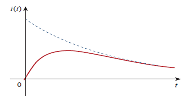
The discriminant vanishes and the roots coincide at \(s_{1} = s_{2} = -\alpha\). Here the naive answer fails, and it is worth seeing why.
Substituting the repeated root into the general form gives
This cannot be right: a single constant \(A_{3}\) cannot satisfy two independent initial conditions. A second, linearly independent solution is missing.
To find it, note that with \(\alpha = \omega_{0}\) the differential equation factors:
Writing \(f = di/dt + \alpha i\) reduces this to a first-order equation \(df/dt + \alpha f = 0\), whose solution is \(f = A_{1}e^{-\alpha t}\). Substituting back and solving the resulting first-order equation produces the missing \(t\) factor:
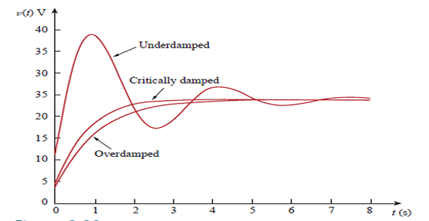
Critical damping is the boundary between the other two cases, and it has a practical significance out of proportion to its narrowness: it is the condition that reaches the final value fastest without any overshoot. Instruments, servo mechanisms, door closers and vehicle suspensions are all designed near it.
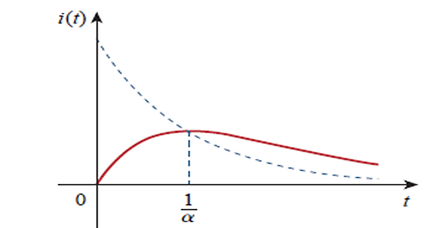
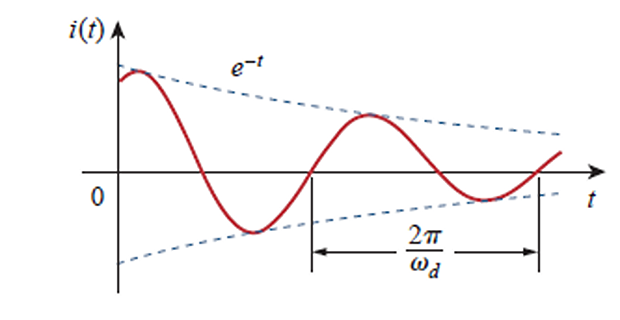
The discriminant is negative, so the roots form a complex conjugate pair:
where \(\omega_{d}\) is the damped natural frequency. Note that \(\omega_{d} < \omega_{0}\) always: damping slows the oscillation as well as decaying it. Using Euler's identity to convert the complex exponentials into trigonometric form:
This is an oscillation of frequency \(\omega_{d}\) inside a decaying envelope \(e^{-\alpha t}\). The circuit rings. Equivalently, combining the two trigonometric terms into a single cosine with a phase angle:
Physically, the energy is being passed back and forth between the capacitor and the inductor faster than the resistance can consume it. Each exchange loses a little, so the amplitude shrinks — but the oscillation persists for many cycles if \(R\) is small. In the limiting case \(R = 0\) we have \(\alpha = 0\), the envelope never decays, and the circuit oscillates forever at \(\omega_{0}\). That is why \(\omega_{0}\) is called the undamped natural frequency, and it is the beginning of the resonance studied in Chapter 14.
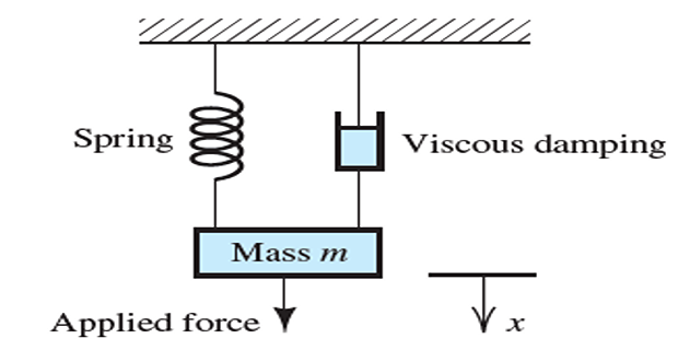
The same three cases appear in every branch of engineering, because the mathematics is identical. A mass on a spring with a damper obeys \(m\ddot{x} + b\dot{x} + kx = 0\), which is the same equation with mass playing the role of inductance, damping the role of resistance and spring compliance the role of capacitance.
A car suspension is the everyday example. Worn dampers give an underdamped ride that bounces after a bump; over-stiff dampers give an overdamped ride that is harsh and slow to recover; the design target is slightly underdamped, close to critical.
Problem. A source-free series RLC circuit has \(L = 1~\mathrm{H}\) and \(C = 40~\mathrm{mF}\), with initial conditions \(i(0) = 4~\mathrm{A}\) and \(v(0) = 0\). Find \(i(t)\) for (a) \(R = 26~\Omega\), (b) \(R = 10~\Omega\), (c) \(R = 6~\Omega\).
Common to all three cases. The resonant frequency depends only on \(L\) and \(C\), so it is the same throughout:
The second initial condition also follows the same pattern, with \(V_{0}=0\):
(a) \(R = 26~\Omega\) — overdamped.
So \(i(t) = A_{1}e^{-t} + A_{2}e^{-25t}\). The two initial conditions give
Substituting \(A_{1} = 4-A_{2}\) into the second: \(-104 = -(4-A_{2})-25A_{2} = -4-24A_{2}\), so \(A_{2} = 25/6\) and \(A_{1} = -1/6\).
(b) \(R = 10~\Omega\) — critically damped.
So \(i(t) = (A_{1}+A_{2}t)e^{-5t}\), with \(A_{1} = i(0) = 4\). Differentiating,
This response crosses zero at exactly \(t = 0.2~\mathrm{s}\) and then approaches zero from below — critical damping permits a single sign change but no oscillation.
(c) \(R = 6~\Omega\) — underdamped.
So \(i(t) = e^{-3t}\left(A_{1}\cos 4t + A_{2}\sin 4t\right)\), with \(A_{1} = i(0) = 4\). Differentiating and setting \(t=0\):
The amplitude form follows from \(\sqrt{4^{2}+3^{2}} = 5\) and \(\tan^{-1}(3/4) = 36.87^{\circ}\). This response genuinely oscillates, crossing zero repeatedly at intervals of \(\pi/\omega_{d} = 0.785~\mathrm{s}\) while the envelope decays.
The comparison is the point. The same \(L\), the same \(C\), the same initial energy — only \(R\) differs, and the behaviour changes from sluggish decay through the fastest clean settling to genuine ringing.
The Source-Free Parallel RLC Circuit
Now put \(R\), \(L\) and \(C\) in parallel. By duality — the theme of Section 8.9 — everything follows the same pattern with current and voltage exchanged.
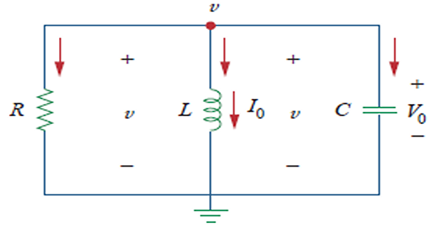
Derivation. Applying KCL at the top node, with the inductor current written as an integral:
Differentiating and dividing by \(C\):
The characteristic equation is \(s^{2} + s/RC + 1/LC = 0\), with the same structure as before but a different \(\alpha\):
Note the crucial difference. In the series circuit \(\alpha = R/2L\) rises with \(R\); in the parallel circuit \(\alpha = 1/2RC\) falls as \(R\) rises. A large resistance damps a series circuit heavily but a parallel circuit hardly at all — which makes sense, since a large parallel resistance draws little current and therefore dissipates little. The resonant frequency \(\omega_{0}\) is unchanged.
The three response forms are identical in shape, with \(v\) in place of \(i\):
| Case | Condition | Parallel-circuit criterion | Response |
|---|---|---|---|
| Overdamped | \(\alpha > \omega_{0}\) | \(L > 4R^{2}C\) | \(v = A_{1}e^{s_{1}t}+A_{2}e^{s_{2}t}\) |
| Critically damped | \(\alpha = \omega_{0}\) | \(L = 4R^{2}C\) | \(v = \left(A_{1}+A_{2}t\right)e^{-\alpha t}\) |
| Underdamped | \(\alpha < \omega_{0}\) | \(L < 4R^{2}C\) | \(v = e^{-\alpha t}\left(A_{1}\cos\omega_{d}t + A_{2}\sin\omega_{d}t\right)\) |
The second initial condition now comes from KCL at \(t = 0\):
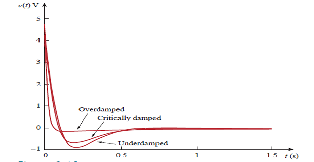
Problem. A source-free parallel RLC circuit has \(L = 1~\mathrm{H}\) and \(C = 10~\mathrm{mF}\), with \(v(0) = 5~\mathrm{V}\) and \(i(0) = 0\). Find \(v(t)\) for (a) \(R = 1.923~\Omega\), (b) \(R = 5~\Omega\), (c) \(R = 6.25~\Omega\).
Common to all.
(a) \(R = 1.923~\Omega\).
With \(v = A_{1}e^{-2t}+A_{2}e^{-50t}\): \(5 = A_{1}+A_{2}\) and \(-260 = -2A_{1}-50A_{2}\), giving
(b) \(R = 5~\Omega\).
With \(v = (A_{1}+A_{2}t)e^{-10t}\): \(A_{1} = 5\), and \(A_{2}-10A_{1} = -100\) gives \(A_{2} = -50\).
(c) \(R = 6.25~\Omega\).
With \(v = e^{-8t}(A_{1}\cos 6t + A_{2}\sin 6t)\): \(A_{1} = 5\), and \(-8A_{1}+6A_{2} = -80\) gives \(A_{2} = -6.667\).
Observe how the parallel circuit behaves oppositely to the series one: here increasing \(R\) moves the circuit from overdamped towards underdamped, whereas in Example 8.2 increasing \(R\) did the reverse.
Step Response of a Series RLC Circuit
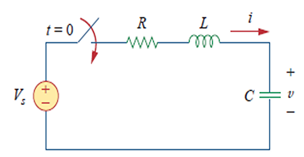
Apply a DC source suddenly and the equation acquires a constant on the right-hand side:
The solution is the sum of two parts, exactly as in Chapter 7:
The steady-state or forced part is simply the final value found from DC analysis, and the natural part takes whichever of the three forms the damping dictates. So:
The constants must be evaluated from the complete response, not from the natural part alone. This is where most errors occur: \(A_{1}\) and \(A_{2}\) are found by imposing \(v(0)\) and \(dv(0)/dt\) on the whole expression including \(V_{s}\).
Find the initial conditions \(x(0)\) and \(dx(0)/dt\) by the methods of Section 8.2, where \(x\) is capacitor voltage or inductor current.
Find the final value \(x(\infty)\) from DC steady state after switching.
Compute \(\alpha\) and \(\omega_{0}\) using the formula appropriate to the topology — series or parallel.
Compare them to classify the damping, and write the corresponding response form with \(x(\infty)\) added.
Impose the two initial conditions on the complete expression to find \(A_{1}\) and \(A_{2}\).
Check: substitute \(t=0\) and confirm the initial value; let \(t\to\infty\) and confirm the final value.
Step 6 costs seconds and catches most algebraic slips. Use it every time.
Problem. A 24 V source is applied at \(t=0\) to a series circuit of \(R = 5~\Omega\), \(L = 1~\mathrm{H}\) and \(C = 0.25~\mathrm{F}\), with a 1 \(\Omega\) resistor across the capacitor carrying the initial conditions. Before switching, \(i(0) = 24/(5+1) = 4~\mathrm{A}\) and \(v(0) = 4~\mathrm{V}\). Find \(v(t)\) and \(i(t)\) for \(t>0\).
Solution. Damping parameters first:
The final value is 24 V, so the complete response is
The first initial condition:
The second comes from the capacitor current, which is the inductor current:
Solving the pair gives \(A_{1} = -64/3\) and \(A_{2} = 4/3\):
Check. At \(t=0\): \(v = 24 + \tfrac{4}{3}(-15) = 24-20 = 4\) V \(\checkmark\) and \(i = \tfrac{4}{3}(3) = 4\) A \(\checkmark\). As \(t\to\infty\): \(v \to 24\) V and \(i \to 0\) \(\checkmark\).
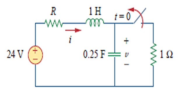
Problem. Repeat Example 8.4 with \(R = 4~\Omega\).
Solution. The initial conditions change with \(R\):
From \(v(0) = 4.8\): \(4.8 = 24 + A_{1}\), so \(A_{1} = -19.2\). From the derivative condition,
Check. At \(t=0\): \(v = 24-19.2 = 4.8\) V \(\checkmark\), \(i = 4.8\) A \(\checkmark\).
Problem. Repeat with \(R = 1~\Omega\).
Solution.
From \(v(0) = 12 = 24 + A_{1}\): \(A_{1} = -12\). The derivative condition:
With \(\zeta = 0.25\) this response overshoots substantially before settling. The percentage overshoot for a second-order step response is
This formula, standard in control engineering, depends on \(\zeta\) alone — not on \(\omega_{0}\), nor on the individual element values. Damping ratio is the single number that determines the shape of the response; \(\omega_{0}\) only sets its speed.
Step Response of a Parallel RLC Circuit
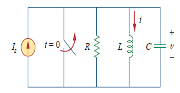
By duality once more, applying a step of current \(I_{s}\) to a parallel RLC circuit gives
where \(i\) is the inductor current. The complete response is
with \(\alpha = 1/2RC\) and \(\omega_{0} = 1/\sqrt{LC}\) as in Section 8.5. The final value is \(I_{s}\), since in DC steady state the inductor becomes a short circuit and takes the entire source current, leaving nothing for \(R\) or \(C\).
The dual pairing is worth writing out explicitly, because it saves memorising a second set of results:
| Series RLC | Parallel RLC |
|---|---|
| Excited by a voltage step \(V_{s}\) | Excited by a current step \(I_{s}\) |
| Solve for capacitor voltage \(v\) | Solve for inductor current \(i\) |
| \(\alpha = R/2L\) | \(\alpha = 1/2RC\) |
| Final value \(v(\infty) = V_{s}\) | Final value \(i(\infty) = I_{s}\) |
| \(dv(0)/dt = i(0)/C\) | \(di(0)/dt = v(0)/L\) |
| Large \(R\) increases damping | Large \(R\) decreases damping |
General Second-Order Circuits
Many second-order circuits are neither purely series nor purely parallel, and no ready-made formula for \(\alpha\) applies. The method then reverts to first principles, but the structure of the solution is unchanged.
Choose a convenient variable — usually a capacitor voltage or inductor current — and apply Kirchhoff's laws to obtain a second-order differential equation in it.
Read \(\alpha\) and \(\omega_{0}\) off by comparing with the standard form \(\ddot{x} + 2\alpha\dot{x} + \omega_{0}^{2}x = f\).
Classify, write the response form, and evaluate the constants exactly as before.
A useful shortcut for source-free circuits: if the network reduces, by series and parallel combination alone, to a single loop or a single node pair, then the standard formulas apply using the equivalent \(R\), \(L\) and \(C\). Only when it does not reduce is the full derivation needed.
Problem. A circuit consists of a 12 \(\Omega\) resistor in series with a 2 H inductor, this combination being in parallel with a 20 mF capacitor. The circuit is source-free with \(v(0) = 10~\mathrm{V}\) across the capacitor and \(i(0) = 0\). Classify the response and find \(v(t)\).
Solution. This is a single loop, so it is effectively a series RLC circuit — the capacitor, inductor and resistor all carry the same current. Hence the series formulas apply:
Working in the capacitor voltage, the initial conditions are \(v(0) = 10\) V and, since the capacitor current equals the (zero) loop current,
The envelope amplitude is \(\sqrt{10^{2}+7.5^{2}} = 12.5\) V, which is larger than the initial 10 V. This is not a contradiction, and it is worth being careful about: 12.5 V is the amplitude of the envelope \(12.5e^{-3t}\), not a value the response ever attains. Because of the \(-36.87^{\circ}\) phase offset the cosine is not at its peak when the envelope is largest, and differentiating confirms that \(dv/dt = -62.5e^{-3t}\sin 4t\), which vanishes at \(t=0\). The response therefore starts at its maximum of 10 V — as it must, since \(dv(0)/dt = 0\) was one of our initial conditions.
An op-amp circuit containing two capacitors is second order, and the same classification applies. Such circuits are the standard way of building active filters, because they achieve second-order responses without inductors — which are bulky, lossy and hard to fabricate on a chip. The Sallen–Key topology of Chapter 14 is the best-known example, and its damping is set by a resistor ratio rather than by a physical inductance.
Duality
Duality has been used informally since Chapter 6. It can be made systematic, and doing so turns every solved problem into two.
Two circuits are duals if the mesh equations of one have the same form as the node equations of the other. Solve one and the other's solution follows by substituting the paired quantities.
| Quantity | Dual | Quantity | Dual |
|---|---|---|---|
| Voltage \(v\) | Current \(i\) | Series | Parallel |
| Resistance \(R\) | Conductance \(G\) | Node | Mesh |
| Inductance \(L\) | Capacitance \(C\) | KVL | KCL |
| Voltage source | Current source | Short circuit | Open circuit |
| Thévenin | Norton | Switch closed | Switch open |
Constructing a dual. For a planar network:
Place a node at the centre of each mesh, and one external node outside the network.
Draw a line between each pair of nodes, crossing exactly one element, and place the dual of that element on the line.
Assign source polarities so that a clockwise mesh current corresponds to a current source directed into the node.
The result explains everything observed in this chapter. The series RLC circuit and the parallel RLC circuit are duals, which is why \(\alpha = R/2L\) becomes \(\alpha = 1/2RC = G/2C\) under the substitutions \(R\to G\) and \(L\to C\). Not a coincidence but a theorem.
Problem. A series RLC circuit has \(R = 5~\Omega\), \(L = 2~\mathrm{H}\), \(C = 0.1~\mathrm{F}\). Construct the element values of its dual parallel circuit and verify that both have the same damping behaviour.
Solution. For the series circuit:
so \(\zeta = 1.25/2.236 = 0.5590\) and the circuit is underdamped.
Under duality, \(R \to G\) numerically, \(L \to C\) and \(C \to L\). The dual parallel circuit therefore has \(G' = 5~\mathrm{S}\) (that is, \(R' = 0.2~\Omega\)), \(C' = 2~\mathrm{F}\) and \(L' = 0.1~\mathrm{H}\). Checking:
Both parameters are identical, so the two circuits have exactly the same damping ratio and the same response shape — one in voltage, the other in current. Anything proved for one is automatically true of the other.
Practical Engineering Applications
The classical ignition circuit is a second-order transient exploited deliberately. An ignition coil of inductance \(L\) and winding resistance \(R\) is connected across the 12 V battery through the contact breaker points, and current builds up according to the RL step response of Chapter 7. When the points open, that current must find another path — and the only one available is the small capacitor deliberately placed across the points.
The inductor and capacitor now form a series RLC circuit with almost no resistance, so the response is heavily underdamped. All the energy stored in the magnetic field transfers into the capacitor's electric field, and since \(\tfrac{1}{2}Li^{2} = \tfrac{1}{2}Cv^{2}\) at the moment of complete transfer, the peak voltage is
The quantity \(\sqrt{L/C}\) has units of ohms and is called the characteristic impedance of the LC pair. It reappears throughout Part 2.
Problem. An ignition coil has \(L = 6~\mathrm{mH}\) and winding resistance \(R = 4~\Omega\), fed from a 12 V battery, with \(C = 1~\mu\mathrm{F}\) across the contact points. Find the steady current, the stored energy, the peak voltage generated when the points open, and the ringing frequency.
Solution. The steady current is set by the winding resistance alone:
When the points open, that energy transfers to the capacitor:
The oscillation frequency is the resonant frequency of the LC pair:
A 12 V battery has produced 232 V — a gain of nearly twenty, purely from the transient. The ignition coil is also a transformer with a turns ratio of about a hundred, so the secondary sees more than 20 kV, which is what jumps the spark-plug gap.
The capacitor is not optional. Without it, \(C \to 0\) makes \(\sqrt{L/C}\) unbounded, and the voltage rises until an arc strikes across the opening points and burns them away. Early mechanics called this component the condenser, and a failed one was a common cause of breakdown.
The reverse problem — suppressing ringing rather than creating it — is just as common. A rectifier feeding an LC filter produces a second-order circuit whose damping must be controlled, or the output will oscillate after every load change. The same applies to a digital signal on a printed-circuit track: track inductance and load capacitance form an underdamped pair, and the resulting overshoot can exceed a logic device's rated input voltage. The standard remedy is a small series termination resistor chosen to bring \(\zeta\) close to 1, trading a little speed for a clean edge — precisely the trade-off illustrated in the response diagram of Section 8.4.
Second-order transients are worth simulating because the effect of changing one element is immediately visible. A parameter sweep over \(R\) reproduces the three cases of Example 8.2 on a single plot:
As in Chapter 7, \(\texttt{UIC}\) instructs the simulator to honour the specified initial conditions rather than computing its own operating point.
Summary and Key Formulas
A second-order circuit has two irreducible storage elements and needs two initial conditions.
Initial values come from continuity; initial derivatives come from \(dv(0)/dt = i_{C}(0)/C\) and \(di(0)/dt = v_{L}(0)/L\); final values from DC steady state.
The characteristic equation is \(s^{2}+2\alpha s+\omega_{0}^{2}=0\), with roots \(s_{1,2} = -\alpha \pm \sqrt{\alpha^{2}-\omega_{0}^{2}}\).
For a series circuit \(\alpha = R/2L\); for a parallel circuit \(\alpha = 1/2RC\). In both, \(\omega_{0} = 1/\sqrt{LC}\).
Three cases: overdamped (\(\alpha>\omega_{0}\), two real roots), critically damped (\(\alpha=\omega_{0}\), repeated root, needs the \(t\) factor), underdamped (\(\alpha<\omega_{0}\), complex pair, oscillates at \(\omega_{d}\)).
Critical damping reaches the final value fastest without overshoot.
The damping ratio \(\zeta = \alpha/\omega_{0}\) determines the shape of the response; \(\omega_{0}\) determines its speed.
A step response is the final value plus the natural response, with the constants evaluated from the complete expression.
Series and parallel RLC circuits are duals, as are voltage and current, \(R\) and \(G\), \(L\) and \(C\), KVL and KCL.
| Result | Formula | Notes |
|---|---|---|
| Characteristic equation | \(s^{2}+2\alpha s+\omega_{0}^{2}=0\) | standard form |
| Natural frequencies | \(s_{1,2} = -\alpha \pm \sqrt{\alpha^{2}-\omega_{0}^{2}}\) | Np/s |
| Series damping factor | \(\alpha = \dfrac{R}{2L}\) | rises with \(R\) |
| Parallel damping factor | \(\alpha = \dfrac{1}{2RC}\) | falls with \(R\) |
| Resonant frequency | \(\omega_{0} = \dfrac{1}{\sqrt{LC}}\) | same for both |
| Damping ratio | \(\zeta = \alpha/\omega_{0}\) | dimensionless |
| Damped frequency | \(\omega_{d} = \sqrt{\omega_{0}^{2}-\alpha^{2}}\) | underdamped only |
| Overdamped | \(A_{1}e^{s_{1}t}+A_{2}e^{s_{2}t}\) | \(\alpha>\omega_{0}\) |
| Critically damped | \(\left(A_{1}+A_{2}t\right)e^{-\alpha t}\) | \(\alpha=\omega_{0}\) |
| Underdamped | \(e^{-\alpha t}\left(A_{1}\cos\omega_{d}t+A_{2}\sin\omega_{d}t\right)\) | \(\alpha<\omega_{0}\) |
| Series 2nd initial condition | \(\dfrac{di(0)}{dt} = -\dfrac{RI_{0}+V_{0}}{L}\) | from KVL |
| Parallel 2nd initial condition | \(\dfrac{dv(0)}{dt} = -\dfrac{v(0)+RI_{0}}{RC}\) | from KCL |
| Derivative conditions | \(\dfrac{dv(0)}{dt} = \dfrac{i_{C}(0)}{C}\), \(\dfrac{di(0)}{dt} = \dfrac{v_{L}(0)}{L}\) | general |
| Step response | \(x(t) = x(\infty) + x_{n}(t)\) | constants from complete form |
| Percentage overshoot | \(100\,e^{-\pi\zeta/\sqrt{1-\zeta^{2}}}\) | depends on \(\zeta\) alone |
| Characteristic impedance | \(\sqrt{L/C}\) | ohms; peak \(V = I\sqrt{L/C}\) |
| Critical \(R\), series | \(R = 2\sqrt{L/C}\) | from \(\alpha=\omega_{0}\) |
Common Mistakes
Using \(\alpha = R/2L\) for a parallel circuit. The parallel value is \(1/2RC\), and the two behave oppositely as \(R\) changes. Identify the topology before reaching for a formula.
Writing \(A_{1}e^{-\alpha t}+A_{2}e^{-\alpha t}\) for the critically damped case. That collapses to a single constant and cannot satisfy two initial conditions. The correct form is \(\left(A_{1}+A_{2}t\right)e^{-\alpha t}\).
Evaluating the constants from the natural response alone in a step problem. The initial conditions apply to the complete response, final value included.
Forgetting the product rule when differentiating. Both \(\left(A_{1}+A_{2}t\right)e^{-\alpha t}\) and \(e^{-\alpha t}\cos\omega_{d}t\) are products; differentiating only one factor loses a term.
Confusing \(\omega_{0}\) with \(\omega_{d}\). The circuit oscillates at \(\omega_{d}\), which is always less than \(\omega_{0}\). They coincide only when \(R=0\).
Assuming two storage elements always give a second-order circuit. Two capacitors that combine into one give a first-order circuit. The elements must be irreducible.
Applying the derivative condition before the continuity condition. You need \(v(0^{+})\) and \(i(0^{+})\) first; the derivatives are computed from the circuit at \(t=0^{+}\) using those values.
Treating \(dx(0)/dt = 0\) as meaning the variable is constant. It means the response is momentarily at a turning point, nothing more.
Mixing radians and degrees in the phase angle. When writing \(Ae^{-\alpha t}\cos(\omega_{d}t+\phi)\), the argument \(\omega_{d}t\) is in radians; state the units of \(\phi\) explicitly.
Expecting critical damping to be achievable in practice. It requires an exact equality between component values that have tolerances. Real designs aim slightly to one side, usually a little underdamped.
Chapter Review
Work these before opening the answers. Always check \(t=0\) and \(t\to\infty\) against your assembled expression.
P8.1 A series RLC circuit has \(R = 10~\Omega\), \(L = 0.5~\mathrm{H}\) and \(C = 2~\mathrm{mF}\). Find \(\alpha\), \(\omega_{0}\), \(\zeta\), and classify the response.
Show answer
\[\alpha = \frac{10}{2(0.5)} = 10, \qquad \omega_{0} = \frac{1}{\sqrt{(0.5)(0.002)}} = \frac{1}{\sqrt{0.001}} = 31.62\]\[\zeta = \frac{10}{31.62} = 0.3162 \;\Longrightarrow\; \text{underdamped}, \qquad \omega_{d} = \sqrt{1000-100} = 30~\mathrm{rad/s}\]P8.2 A source-free series RLC circuit has \(R = 25~\Omega\), \(L = 1~\mathrm{H}\), \(C = 10~\mathrm{mF}\), with \(i(0) = 2~\mathrm{A}\) and \(v(0) = 0\). Find \(i(t)\).
Show answer
\[\alpha = 12.5, \quad \omega_{0} = 10 \;\Longrightarrow\; \text{overdamped}, \quad s_{1,2} = -12.5 \pm 7.5 = -5, \; -20\]From \(A_1+A_2 = 2\) and \(-5A_1-20A_2 = -50\): \(A_1 = -2/3\), \(A_2 = 8/3\).\[\frac{di(0)}{dt} = -\frac{(25)(2)+0}{1} = -50\]\[i(t) = -\tfrac{2}{3}e^{-5t} + \tfrac{8}{3}e^{-20t}~\mathrm{A}\]P8.3 What value of \(R\) gives critical damping in a series circuit with \(L = 4~\mathrm{H}\) and \(C = 1~\mathrm{mF}\)?
Show answer
Setting \(\alpha = \omega_{0}\) gives \(R/2L = 1/\sqrt{LC}\), so\[R = 2\sqrt{\frac{L}{C}} = 2\sqrt{\frac{4}{0.001}} = 2\sqrt{4000} = 126.5~\Omega\]P8.4 A parallel RLC circuit has \(R = 10~\Omega\) and \(C = 5~\mathrm{mF}\). What \(L\) makes it critically damped?
Show answer
Critical damping requires \(L = 4R^{2}C\):Check: \(\alpha = 1/(2\times10\times0.005) = 10\) and \(\omega_{0} = 1/\sqrt{(2)(0.005)} = 10\) \(\checkmark\)\[L = 4(100)(0.005) = 2.000~\mathrm{H}\]P8.5 A 20 V step is applied to a series circuit with \(R = 6~\Omega\), \(L = 1~\mathrm{H}\), \(C = 40~\mathrm{mF}\), initially at rest. Find \(v(t)\) across the capacitor.
Show answer
\[\alpha = 3, \quad \omega_{0} = 5 \;\Longrightarrow\; \text{underdamped}, \quad \omega_{d} = 4\]With \(v(0)=0\): \(A_1 = -20\). With \(dv(0)/dt = i(0)/C = 0\): \(-3(-20)+4A_2 = 0\), so \(A_2 = -15\).\[v(t) = 20 + e^{-3t}\left(A_{1}\cos 4t + A_{2}\sin 4t\right)\]At \(t = 0.5~\mathrm{s}\): \(v = 18.81~\mathrm{V}\).\[v(t) = 20 - e^{-3t}\left(20\cos 4t + 15\sin 4t\right)~\mathrm{V}\]P8.6 For P8.5, find the damping ratio and the percentage overshoot.
Show answer
\[\zeta = \frac{3}{5} = 0.6000\]\[\%\,\text{OS} = 100\,e^{-\pi(0.6)/\sqrt{1-0.36}} = 100\,e^{-\pi(0.6)/0.8} = 100\,e^{-2.356} = 9.478\,\%\]P8.7 A circuit has \(v(0^{-}) = 6~\mathrm{V}\) across a 0.2 F capacitor and \(i(0^{-}) = 3~\mathrm{A}\) through a 0.5 H inductor. At \(t=0^{+}\) the capacitor current is 3 A and the inductor voltage is \(-4~\mathrm{V}\). Find both initial derivatives.
Show answer
\[\frac{dv(0^{+})}{dt} = \frac{i_{C}(0^{+})}{C} = \frac{3}{0.2} = 15.00~\mathrm{V/s}\]\[\frac{di(0^{+})}{dt} = \frac{v_{L}(0^{+})}{L} = \frac{-4}{0.5} = -8.000~\mathrm{A/s}\]P8.8 Construct the dual element values for a parallel RLC circuit with \(R = 4~\Omega\), \(L = 0.5~\mathrm{H}\), \(C = 0.25~\mathrm{F}\), and verify that \(\alpha\) and \(\omega_{0}\) match.
Show answer
Original: \(\alpha = 1/(2\times4\times0.25) = 0.5\), \(\omega_{0} = 1/\sqrt{0.125} = 2.828\).
Dual series circuit: \(R' = 1/4 = 0.25~\Omega\), \(L' = 0.25~\mathrm{H}\), \(C' = 0.5~\mathrm{F}\).\[\alpha' = \frac{0.25}{2(0.25)} = 0.5 \;\checkmark, \qquad \omega_{0}' = \frac{1}{\sqrt{(0.25)(0.5)}} = \frac{1}{\sqrt{0.125}} = 2.828 \;\checkmark\]P8.9 An underdamped circuit has \(\alpha = 2\) and \(\omega_{d} = 6~\mathrm{rad/s}\). Find \(\omega_{0}\), \(\zeta\), and the interval between successive zero crossings.
Show answer
\[\omega_{0} = \sqrt{\alpha^{2}+\omega_{d}^{2}} = \sqrt{4+36} = \sqrt{40} = 6.325~\mathrm{rad/s}\]\[\zeta = \frac{2}{6.325} = 0.3162, \qquad \Delta t = \frac{\pi}{\omega_{d}} = \frac{\pi}{6} = 0.5236~\mathrm{s}\]P8.10 An ignition coil has \(L = 8~\mathrm{mH}\) carrying 4 A, with \(C = 0.5~\mu\mathrm{F}\) across the points. Find the stored energy and the peak voltage.
Show answer
\[w = \tfrac{1}{2}\left(8\times10^{-3}\right)(16) = 64.00~\mathrm{mJ}\]\[V_{\text{peak}} = I\sqrt{\frac{L}{C}} = 4\sqrt{\frac{8\times10^{-3}}{0.5\times10^{-6}}} = 4\sqrt{16\,000} = 4(126.5) = 505.9~\mathrm{V}\]
MCQ 1. For a series RLC circuit the damping factor is:
(a) \(1/2RC\) (b) \(R/2L\) (c) \(2L/R\) (d) \(1/\sqrt{LC}\)Show answer
(b) \(R/2L\). Option (a) is the parallel case and (d) is \(\omega_{0}\).MCQ 2. A circuit is underdamped when:
(a) \(\alpha > \omega_{0}\) (b) \(\alpha = \omega_{0}\) (c) \(\alpha < \omega_{0}\) (d) \(\alpha = 0\)Show answer
(c) \(\alpha < \omega_{0}\), giving complex roots and oscillation.MCQ 3. The critically damped response has the form:
(a) \(A_{1}e^{s_{1}t}+A_{2}e^{s_{2}t}\) (b) \(\left(A_{1}+A_{2}t\right)e^{-\alpha t}\) (c) \(Ae^{-\alpha t}\) (d) \(e^{-\alpha t}\cos\omega_{d}t\)Show answer
(b). Option (c) has only one constant and cannot meet two initial conditions.MCQ 4. A series RLC circuit has \(R=4~\Omega\), \(L=1~\mathrm{H}\), \(C=0.25~\mathrm{F}\). The response is:
(a) overdamped (b) critically damped (c) underdamped (d) undampedShow answer
(b) critically damped. \(\alpha = 2\) and \(\omega_{0} = 1/\sqrt{0.25} = 2\).MCQ 5. The damped natural frequency \(\omega_{d}\) is always:
(a) greater than \(\omega_{0}\) (b) less than \(\omega_{0}\) (c) equal to \(\omega_{0}\) (d) equal to \(\alpha\)Show answer
(b) less than \(\omega_{0}\), since \(\omega_{d} = \sqrt{\omega_{0}^{2}-\alpha^{2}}\). They are equal only when \(R=0\).MCQ 6. Increasing \(R\) in a parallel RLC circuit:
(a) increases damping (b) decreases damping (c) leaves damping unchanged (d) changes \(\omega_{0}\)Show answer
(b) decreases damping, since \(\alpha = 1/2RC\) falls as \(R\) rises. The opposite of the series case.MCQ 7. The response that reaches its final value fastest without overshoot is:
(a) overdamped (b) critically damped (c) underdamped (d) undampedShow answer
(b) critically damped — which is why instruments and servos are designed near it.MCQ 8. The dual of inductance is:
(a) resistance (b) conductance (c) capacitance (d) impedanceShow answer
(c) capacitance. Voltage pairs with current, \(R\) with \(G\), and \(L\) with \(C\).MCQ 9. The initial derivative of capacitor voltage is found from:
(a) \(v(0)/R\) (b) \(i_{C}(0)/C\) (c) \(v_{L}(0)/L\) (d) \(Ci_{C}(0)\)Show answer
(b) \(i_{C}(0)/C\), from \(i = C\,dv/dt\). Option (c) gives the inductor-current derivative.MCQ 10. A second-order circuit with \(R = 0\) would:
(a) not respond (b) be critically damped (c) oscillate forever at \(\omega_{0}\) (d) be overdampedShow answer
(c) oscillate forever at \(\omega_{0}\). With \(\alpha = 0\) the envelope never decays — the undamped case, and the starting point for resonance in Chapter 14.
Explain physically why a series RLC circuit becomes more damped as \(R\) increases while a parallel one becomes less damped.
The critically damped solution requires an extra factor of \(t\). Explain why the naive two-exponential form fails, without reproducing the algebra.
Why does the damping ratio \(\zeta\) determine the shape of a response while \(\omega_{0}\) determines only its speed? What does this imply for scaling a design to a different frequency?
An underdamped circuit oscillates even though it contains no source. Where does the energy for each successive half-cycle come from, and why does the amplitude shrink?
Critical damping is often described as the ideal design target, yet it is never exactly achieved. Explain why, and say which side of it you would err towards for (a) a measuring instrument and (b) a digital signal line.
The ignition circuit deliberately produces a large transient voltage, while a digital termination resistor deliberately suppresses one. Both are second-order problems. What single parameter is being adjusted in opposite directions?
Part 1 ends here. Every source since Chapter 1 has been DC, and the interest has been in what happens during the brief interval after a switch operates. From Chapter 9 the sources become sinusoidal, and the interest shifts to the steady state that persists indefinitely.
That change of emphasis brings an enormous simplification. Solving a differential equation for a sinusoidal input is laborious; but if only the steady state is wanted, the phasor converts every derivative into a multiplication and every differential equation into an algebraic one. The whole apparatus of Chapters 2 to 4 — Ohm's law, nodal and mesh analysis, Thévenin and Norton — returns unchanged, with complex numbers in place of real ones.
The parameter \(\omega_{0}\) defined in this chapter will reappear as the frequency at which a circuit responds most strongly, and the damping ratio as the quantity governing how sharp that response is. What was a transient here becomes resonance there.