- Recognise a first-order circuit and identify which of the four possible cases applies.
- Derive and use the natural response of the source-free RC and RL circuits.
- Compute the time constant from the Thévenin resistance seen by the storage element, and interpret it physically.
- Use the unit step, impulse and ramp functions to describe switching and to build pulses.
- Determine the step response of RC and RL circuits.
- Apply the universal first-order formula to any first-order circuit from three quantities.
- Separate a complete response into transient and steady-state, or natural and forced, parts.
- Analyse first-order circuits containing operational amplifiers.
- Explain how RC timing underlies delay circuits, photoflash units and relay drivers.
Introduction
Chapter 6 introduced the capacitor and the inductor but stopped short of putting either into a circuit and solving it. That is the business of this chapter. A first-order circuit contains exactly one energy-storage element together with resistance, and is so named because applying Kirchhoff's laws to it produces a first-order differential equation.
Because there is only one storage element, there are only two kinds of first-order circuit — the RC circuit and the RL circuit. And because there are only two ways to put energy into a circuit, there are only four situations to master in total:
| Excitation | RC circuit | RL circuit |
|---|---|---|
| Source-free — energy already stored in the element | Section 7.2 | Section 7.4 |
| Step — an independent source suddenly applied | Section 7.6 | Section 7.7 |
The two forms of excitation deserve their names. In the natural response the circuit is free of independent sources; whatever energy was stored in the capacitor or inductor drives a current that the resistors gradually dissipate, and the circuit relaxes to rest. A source-free circuit may still contain dependent sources — "source-free" means no independent sources. In the forced response an independent source, usually DC here, drives the circuit to a new condition.
The remarkable thing — established in Section 7.8 — is that all four cases collapse into a single formula requiring three numbers. Work through the derivations first, because the formula means little without them, but do not lose sight of where this is heading.
The Source-Free RC Circuit
A source-free RC circuit arises whenever a charged capacitor is suddenly disconnected from its supply and left connected to a resistance. The energy stored in the capacitor is released into the resistor and dissipated as heat.
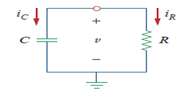
Derivation. Let the initial capacitor voltage be
Apply KCL at the top node. The capacitor current and the resistor current must sum to zero:
This is the first-order differential equation the chapter is named for. Divide by \(C\) and separate the variables:
Integrating both sides, with \(\ln A\) as the constant of integration:
The constant follows from the initial condition. At \(t = 0\) the exponential is unity, so \(A = V_{0}\), giving the natural response:
The voltage decays exponentially from its initial value towards zero. Note that we could write down the initial condition immediately only because capacitor voltage is continuous — the property established in Section 6.3. Without it there would be no way to connect the circuit's state before the switching to its state after.
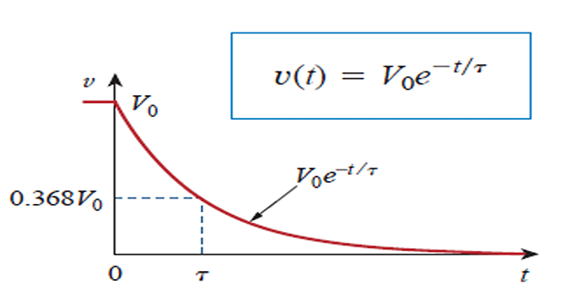
Everything else in the circuit follows at once:
Observe that the power decays at twice the rate of the voltage, since it depends on the square.
The Time Constant
The rate at which the response decays is set entirely by the product \(RC\), called the time constant and denoted \(\tau\). Its definition is worth stating precisely:
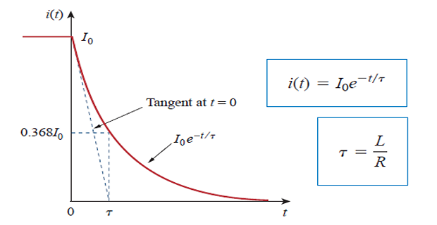
The time constant is the time required for the response to decay to \(1/e\) — that is, 36.8 % — of its initial value. Setting \(t = \tau\) confirms it:
Despite being a product of ohms and farads, \(\tau\) has units of seconds — as it must, since it appears in the exponent alongside \(t\). A quick check: \(\Omega \cdot \mathrm{F} = (\mathrm{V/A})(\mathrm{C/V}) = \mathrm{C/A} = \mathrm{s}\).
| Time | \(e^{-t/\tau}\) | Decayed to | Elapsed |
|---|---|---|---|
| \(\tau\) | 0.3679 | 36.79 % | 63.21 % complete |
| \(2\tau\) | 0.1353 | 13.53 % | 86.47 % complete |
| \(3\tau\) | 0.0498 | 4.98 % | 95.02 % complete |
| \(4\tau\) | 0.0183 | 1.83 % | 98.17 % complete |
| \(5\tau\) | 0.0067 | 0.67 % | 99.33 % complete |
This table justifies a rule used throughout engineering: after five time constants the response is within 1 % of its final value, and the circuit is taken as fully settled. The exponential never mathematically reaches zero, but after \(5\tau\) the remaining difference is smaller than the tolerance of any component in the circuit.
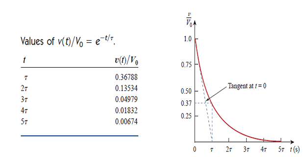
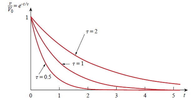
There is also a neat geometrical reading. The tangent to the curve at \(t = 0\) has slope \(-V_{0}/\tau\), so if the response continued to fall at its initial rate it would reach zero exactly at \(t = \tau\). This gives a practical way to measure \(\tau\) from an oscilloscope trace.
Find the initial capacitor voltage \(v(0)\), usually from the DC steady state before the switch operates, using continuity: \(v(0^{+}) = v(0^{-})\).
Find the time constant \(\tau = R_{Th}C\), where \(R_{Th}\) is the Thévenin resistance seen by the capacitor after switching, with the capacitor removed.
Write down \(v(t) = v(0)e^{-t/\tau}\), and obtain any other quantity from it.
Step 2 is where Chapter 4 pays off. The capacitor rarely faces a single resistor; it faces a network, and the relevant resistance is the Thévenin resistance of that network looking back from the capacitor's terminals. Everything you learned about finding \(R_{Th}\) applies unchanged.
Problem. A \(10~\mu\mathrm{F}\) capacitor charged to 20 V is discharged through a \(5~\mathrm{k}\Omega\) resistor. Find \(\tau\), \(v(t)\), \(i(t)\), the initial stored energy, and the time for the voltage to fall to 5 V.
Solution.
For the time to reach 5 V, take logarithms:
Note that falling to a quarter takes \(\ln 4 = 1.386\) time constants, and the circuit is fully discharged for practical purposes after \(5\tau = 250~\mathrm{ms}\).
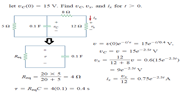
Problem. A 24 V source in series with a 4 \(\Omega\) resistor feeds node \(A\). From \(A\), a 12 \(\Omega\) and a 6 \(\Omega\) resistor run to ground in parallel, and a 50 mF capacitor is also connected from \(A\) to ground. The switch has been closed a long time; at \(t = 0\) it opens, disconnecting the source and the 4 \(\Omega\). Find \(v(t)\) for \(t > 0\) and its value at \(t = 0.3~\mathrm{s}\).
Step 1 — the initial condition. For \(t < 0\) the circuit is in DC steady state, so the capacitor is an open circuit (Section 6.8). The two shunt resistors combine:
and a voltage divider gives the node voltage:
By continuity of capacitor voltage, \(v(0^{+}) = v(0^{-}) = 12~\mathrm{V}\).
Step 2 — the time constant. After the switch opens, the source and the 4 \(\Omega\) are gone. Looking out from the capacitor's terminals, it sees only the 12 \(\Omega\) and 6 \(\Omega\) in parallel:
Step 3 — write the response.
The initial stored energy was \(\tfrac{1}{2}(50\times10^{-3})(144) = 3.600~\mathrm{J}\), all of which ends up as heat in the two resistors. A warning about Step 2: the resistance that matters is the one present after switching, not before. Using the pre-switch network — which would have included the 4 \(\Omega\) — is the most common error in this type of problem.
The Source-Free RL Circuit
The dual situation is an inductor carrying current, suddenly left to discharge into a resistance. Everything runs parallel to Section 7.2, with current in place of voltage.
Derivation. Let the initial inductor current be
Apply KVL around the loop. The inductor voltage and the resistor voltage must sum to zero:
Separating variables and integrating exactly as before:
Note the time constant carefully. For the RC circuit it was a product, \(RC\); here it is a quotient, \(L/R\). A large resistance makes an RC circuit slow but an RL circuit fast. Confusing the two is among the most frequent errors in this chapter, and the units settle it: \(\mathrm{H}/\Omega = (\mathrm{V\cdot s/A})/(\mathrm{V/A}) = \mathrm{s}\) \(\checkmark\).
Again the initial condition could be carried across the switching instant only because inductor current is continuous. The associated quantities follow:
Problem. A 2 H inductor carrying 6 A is suddenly connected across an 8 \(\Omega\) resistor. Find \(\tau\), \(i(t)\), the resistor voltage, the initial stored energy, and the time for the current to fall to 1 A.
Solution.
For the current to reach 1 A:
The initial resistor voltage is 48 V — considerably more than you might expect from a circuit with no source in it at all. This is the inductor's stored energy asserting itself, and with a larger resistance it would be larger still, which is the mechanism behind the 50 kV of Practice Problem P6.10.
Problem. A 24 V source in series with a 4 \(\Omega\) resistor feeds node \(A\). A 0.6 H inductor runs from \(A\) to ground, and a 12 \(\Omega\) resistor is also connected from \(A\) to ground. The switch has been closed a long time and opens at \(t = 0\), removing the source and the 4 \(\Omega\). Find \(i(t)\) for \(t > 0\) and its value at \(t = 0.1~\mathrm{s}\).
Step 1 — the initial condition. For \(t < 0\) the circuit is in DC steady state, so the inductor is a short circuit. It therefore short-circuits the 12 \(\Omega\) resistor as well, and the entire source current flows through it:
By continuity of inductor current, \(i(0^{+}) = 6~\mathrm{A}\).
Step 2 — the time constant. After the switch opens, the inductor sees only the 12 \(\Omega\):
Step 3 — the response.
At the instant of switching, the 12 \(\Omega\) resistor must suddenly carry the full 6 A, so the voltage across it jumps from 0 V to 72 V instantaneously. The inductor's current is continuous; its voltage is not. This jump is real and is why inductive circuits damage switches.

Singularity Functions
Before turning to step responses we need a compact notation for switching. Singularity functions are discontinuous functions, or functions with discontinuous derivatives, that describe abrupt events. Three of them matter here, and each is the derivative of the next.
The unit step \(u(t)\) is zero for negative time and one for positive time:
It is undefined exactly at \(t = 0\), where it jumps. Shifting the argument moves the jump:
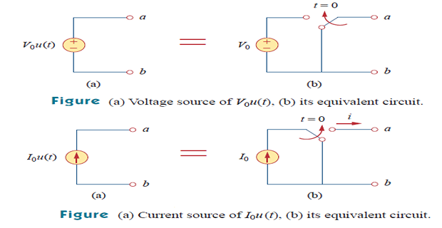
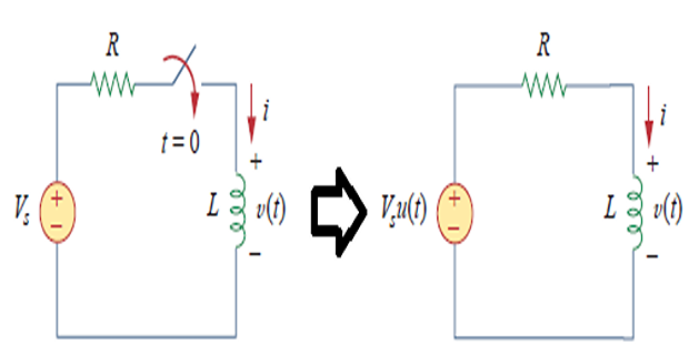
The step is the natural way to represent a switch. A DC source \(V_{s}\) connected at \(t = t_{0}\) is simply \(V_{s}u(t-t_{0})\), and the awkward business of writing "for \(t<0\) … for \(t>0\) …" disappears into a single expression.
Steps also combine to build pulses. A rectangular pulse of height \(A\) lasting from \(t_{1}\) to \(t_{2}\) is the difference of two steps:
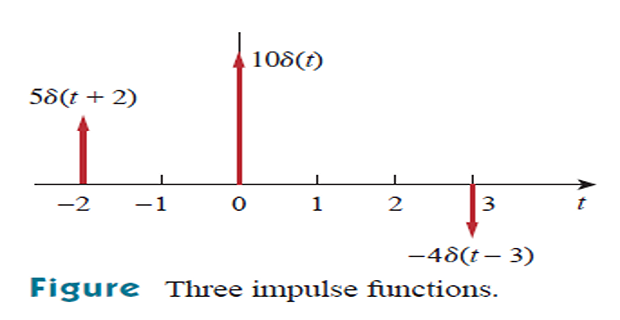
Differentiating the step gives the unit impulse or delta function \(\delta(t)\):
Since the step jumps by one in zero time, its derivative is zero everywhere except at the origin, where it is infinite. What tames this is that the area is finite and equal to one:
The impulse is best thought of as a spike of unit area and vanishing width. Its most useful property is sifting: multiplying any continuous function by an impulse and integrating simply picks out the value of that function at the impulse's location:
No physical source produces a true impulse, but a very short, very large pulse behaves like one, and the idealisation is enormously convenient. It becomes central in Chapter 15, where the impulse response characterises an entire circuit.
Integrating the step instead of differentiating it gives the unit ramp:
The ramp rises linearly with unit slope from the origin. It models a quantity that increases steadily from the moment of switching — the output of the integrator in Example 6.10, for instance.
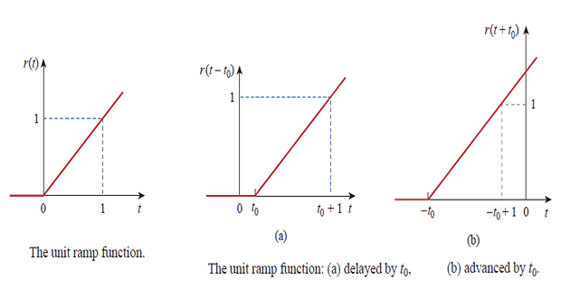
The three form a differentiation chain, and it is worth committing the order to memory:
Problem. Write expressions for (a) a 10 V pulse existing from \(t = 2~\mathrm{s}\) to \(t = 5~\mathrm{s}\), and (b) a waveform that is 0 before \(t=0\), rises linearly at 3 V/s from \(t = 0\), and is switched off at \(t = 4~\mathrm{s}\). Evaluate \(\int_{-\infty}^{\infty}\left(t^{2}+3\right)\delta(t-2)\,dt\).
Solution (a). The pulse turns on at 2 s and off at 5 s, so it is the difference of two shifted steps:
Check at \(t = 3\): the first step is 1, the second still 0, giving \(10(1-0) = 10\) V \(\checkmark\). At \(t = 6\): both are 1, giving \(10(1-1) = 0\) \(\checkmark\).
Solution (b). A ramp of slope 3, truncated at 4 s:
At \(t = 4^{-}\) the value is 12 V, and it drops abruptly to zero.
Solution (c). By the sifting property, the integral simply evaluates the function at \(t = 2\):
No integration is performed at all — the impulse does the work.
Step Response of an RC Circuit
Now a DC source is suddenly applied to an RC circuit — the switch closes rather than opens. The response is called the step response.
Derivation. With a source \(V_{s}\) applied through \(R\) at \(t = 0\) and an initial capacitor voltage \(V_{0}\), KCL gives
This differs from the source-free equation only by the constant on the right. Separating variables:
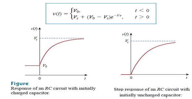
At \(t = 0\) the capacitor voltage is \(V_{0}\), so \(A = V_{0} - V_{s}\) and
For the common case of an initially uncharged capacitor, \(V_{0} = 0\) and this reduces to the familiar charging curve:
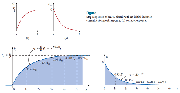
Note the asymmetry: the voltage rises exponentially towards \(V_{s}\) while the current falls exponentially from \(V_{s}/R\) towards zero. At the first instant the uncharged capacitor behaves like a short circuit; after a long time it behaves like an open circuit.
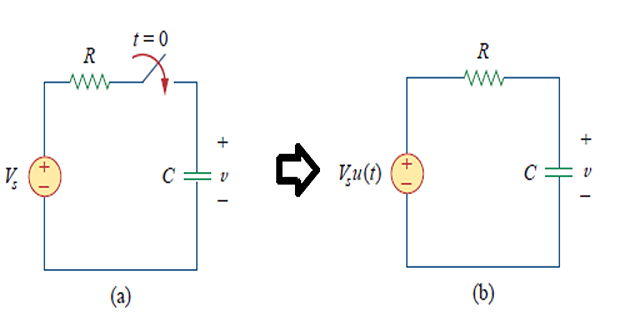
The result above can be decomposed in two different and equally valid ways, and both are used in practice.
Natural plus forced — classified by cause:
Transient plus steady-state — classified by persistence:
The transient response is the part that dies away with time; the steady-state response is how the circuit behaves long after the excitation was applied. Adding either pair reproduces the same total, so the split is a matter of viewpoint rather than physics. The transient/steady-state division is generally the more useful, and it is the one that generalises to sinusoidal excitation in Part 2.
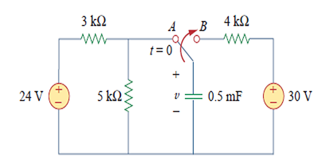
Problem. The switch has been in position \(A\) for a long time, where the capacitor sees a 24 V source across a 3 \(\mathrm{k}\Omega\) and 5 \(\mathrm{k}\Omega\) divider, with the capacitor across the 5 \(\mathrm{k}\Omega\). At \(t = 0\) the switch moves to position \(B\), connecting the \(0.5~\mathrm{mF}\) capacitor to a 30 V source through 4 \(\mathrm{k}\Omega\). Determine \(v(t)\) for \(t > 0\), and evaluate it at \(t = 1~\mathrm{s}\) and \(t = 4~\mathrm{s}\).
Step 1 — initial value. In position \(A\) the circuit has settled, so the capacitor is an open circuit and the divider determines its voltage:
Step 2 — final value. After a long time in position \(B\) the capacitor is again an open circuit, so no current flows through the 4 \(\mathrm{k}\Omega\) and there is no drop across it:
Step 3 — time constant.
Step 4 — assemble.
Evaluating:
Sanity checks: at \(t=0\) the formula gives \(30-15 = 15\) V \(\checkmark\), and as \(t\to\infty\) it gives 30 V \(\checkmark\). The capacitor charges the rest of the way from 15 V to 30 V, and after \(5\tau = 10\) s it is there for all practical purposes.
Step Response of an RL Circuit
The RL step response follows by duality, with current replacing voltage throughout. Applying KVL after the switch closes:
Solving exactly as before, with initial current \(I_{0}\) and final current \(V_{s}/R\):
For an inductor initially at rest, \(I_{0} = 0\) and
Again the roles are exchanged relative to the RC case: here it is the current that rises and the voltage that decays. At the first instant an inductor initially at rest behaves like an open circuit — it refuses to let current start — and after a long time it behaves like a short circuit.
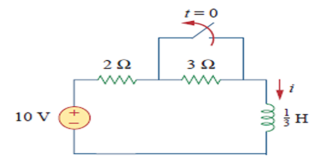
Problem. A 10 V source drives a 2 \(\Omega\) resistor in series with a 0.5 H inductor; a 3 \(\Omega\) resistor is short-circuited by a switch that has been closed a long time. At \(t = 0\) the switch opens, placing the 3 \(\Omega\) in series as well. Find \(i(t)\) for \(t > 0\), the inductor voltage, and \(i\) at \(t = 0.2~\mathrm{s}\).
Step 1 — initial value. With the switch closed and the circuit settled, the inductor is a short and the 3 \(\Omega\) is bypassed:
Step 2 — final value. After the switch opens and the circuit settles again, the inductor is once more a short, but now both resistors are in the path:
Step 3 — time constant. The resistance seen by the inductor after switching is
Step 4 — assemble.
Here the current falls from 5 A to 2 A, so this is a step response with a decreasing output — a reminder that "step response" refers to the excitation being a step, not to the response rising. The formula handles both cases without modification.
The Universal First-Order Formula
Look back at the four results derived so far. Every one of them has the same shape, and that shape can be stated once and applied to all of them:
where \(x\) is capacitor voltage or inductor current — the continuous variable — and the three ingredients are:
| Ingredient | How to find it | Uses |
|---|---|---|
| \(x(0)\) — initial value | DC steady state before switching, then apply continuity | C open, L short (Section 6.8) |
| \(x(\infty)\) — final value | DC steady state after switching | C open, L short again |
| \(\tau\) — time constant | \(R_{Th}C\) or \(L/R_{Th}\), with \(R_{Th}\) seen by the element after switching | Thévenin (Chapter 4) |
No differential equation need ever be solved again for a first-order circuit. Find three numbers using techniques from earlier chapters, and substitute.
Delayed switching. If the switch operates at \(t = t_{0}\) rather than at the origin, the response is simply shifted:
Other quantities. The formula applies directly only to capacitor voltage and inductor current, because only those are guaranteed continuous. To find any other voltage or current, first obtain the continuous variable, then work outwards using Ohm's and Kirchhoff's laws. Applying the formula directly to, say, a resistor current can give the wrong initial value, because that current may well jump at \(t=0\).
First-Order Op Amp Circuits
An op-amp circuit containing a single capacitor is still a first-order circuit, and the universal formula still applies. The only new work is finding the effective time constant, and here the two golden rules of Chapter 5 do it for us.
Consider an inverting amplifier in which the feedback resistor \(R_{f}\) has a capacitor \(C\) in parallel with it, driven through \(R_{1}\) by a step of height \(V_{s}\).
Because the inverting terminal is a virtual ground, the capacitor sees exactly \(R_{f}\) across it — nothing else in the circuit is connected to both its terminals. Hence
The initial value is zero if the capacitor starts uncharged, since the output must equal the (zero) capacitor voltage at that instant. The final value is the ordinary inverting-amplifier gain, because in DC steady state the capacitor is an open circuit and only \(R_{f}\) remains:
Substituting into the universal formula:
The circuit behaves as an amplifier at DC and as an integrator at high frequencies, which makes it a practical compromise between the two: unlike the pure integrator of Section 6.9, its DC gain is finite, so input offsets do not accumulate without limit.
Problem. An inverting amplifier has \(R_{1} = 10~\mathrm{k}\Omega\) and \(R_{f} = 50~\mathrm{k}\Omega\) with a \(2~\mu\mathrm{F}\) capacitor across \(R_{f}\), on \(\pm15~\mathrm{V}\) supplies. A 1 V step is applied at \(t = 0\) with the capacitor uncharged. Find \(v_{o}(t)\) and its value at \(t = 0.15~\mathrm{s}\).
Solution. The three ingredients:
Substituting into the universal formula:
The final value of \(-5\) V is comfortably within the \(\pm15\) V rails, so the linear analysis holds throughout — the saturation check from Chapter 5 has not been forgotten. Contrast this with the pure integrator of Example 6.10, whose output ramped without limit until it hit a rail; adding \(R_{f}\) gives the circuit a finite DC gain and a well-defined final value.
Practical Engineering Applications
The exponential charging of a capacitor gives a simple and reliable way of measuring time. A capacitor charges through a resistor until its voltage reaches a threshold, at which point a switching device — a neon lamp, a comparator, or the trigger input of a 555 timer — fires. The delay is set by \(\tau = RC\) and the threshold fraction:
For an initially uncharged capacitor charging towards \(V_{s}\) and triggering at half the supply, the delay is \(RC\ln 2 = 0.693\,RC\) — a number that appears in every 555 timer design.
The strength of the method is that the threshold is a fraction of the supply, so the delay is independent of supply voltage. Its weakness is that \(R\) and \(C\) both have wide tolerances and drift with temperature, so RC timing is fine for a windscreen-wiper interval and useless for a clock.
Problem. A photoflash capacitor of \(2000~\mu\mathrm{F}\) is charged to 240 V through a 1 \(\mathrm{k}\Omega\) resistor, then discharged through a flash lamp of resistance 10 \(\Omega\). Find the charging and discharging time constants, the stored energy, the peak discharge current, and the average power delivered to the lamp.
Solution. The two time constants differ enormously, which is the whole point of the design:
Taking the flash as lasting \(5\tau_{\text{discharge}} = 0.1~\mathrm{s}\), the average power is
This is the essential trick of a photoflash, and of a defibrillator, a spot welder and a railgun alike: energy is accumulated slowly at low power and released quickly at high power. Here 57.6 J is gathered over ten seconds at an average of only 5.76 W, then dumped in a tenth of a second at 576 W — a power gain of a hundred, which is exactly the ratio of the two time constants. The capacitor is an energy buffer that decouples the rate of supply from the rate of demand.
A relay coil is an inductor, and switching it off is where the RL natural response becomes a practical hazard. When the drive transistor turns off, it attempts to interrupt the coil current in a fraction of a microsecond. Since inductor current cannot change instantaneously, the coil generates whatever voltage is required to keep it flowing — and that voltage will destroy the transistor.
The remedy is a freewheeling diode connected across the coil, reverse-biased in normal operation. When the transistor turns off, the diode becomes forward-biased and provides a path for the current, which then decays with time constant \(L/R_{\text{coil}}\), harmlessly dissipating the stored energy in the coil's own resistance. Every relay, solenoid and motor driven from a semiconductor switch has one.
Transient analysis is where simulation earns its keep, because the waveform is easier to read than the algebra. In SPICE, a switched RC circuit is described with a pulse source and a transient sweep:
The \(\texttt{UIC}\) flag — "use initial conditions" — tells the simulator to honour the initial capacitor voltage you specify rather than computing its own DC operating point, which is exactly what you want when reproducing a hand-worked switching problem.
Summary and Key Formulas
A first-order circuit contains one storage element and is described by a first-order differential equation. There are four cases: RC or RL, source-free or step-excited.
The source-free RC response is \(v = V_{0}e^{-t/\tau}\) with \(\tau = RC\); the source-free RL response is \(i = I_{0}e^{-t/\tau}\) with \(\tau = L/R\).
The time constant is the time to decay to 36.8 % of the initial value; after \(5\tau\) the response is within 1 % of its final value.
Singularity functions describe switching: \(u(t)\), its derivative \(\delta(t)\), and its integral \(r(t)\). The impulse has unit area and the sifting property.
A complete response splits either into natural plus forced, or into transient plus steady-state.
The universal formula \(x(t) = x(\infty)+[x(0)-x(\infty)]e^{-t/\tau}\) solves every first-order circuit from three numbers.
It applies to capacitor voltage and inductor current, the continuous variables; other quantities are found from them afterwards.
\(R_{Th}\) is the Thévenin resistance seen by the storage element after switching.
RC timing underlies delay circuits; RL switching requires freewheeling protection.
| Result | Formula | Notes |
|---|---|---|
| RC time constant | \(\tau = R_{Th}C\) | product |
| RL time constant | \(\tau = L/R_{Th}\) | quotient — do not confuse |
| RC natural response | \(v = V_{0}e^{-t/\tau}\) | source-free |
| RL natural response | \(i = I_{0}e^{-t/\tau}\) | source-free |
| Decay at one \(\tau\) | \(e^{-1} = 0.368\) | 36.8 % remains |
| Settling time | \(5\tau\) | within 1 % |
| Unit step | \(u(t-t_{0})\) | 0 before, 1 after |
| Pulse | \(A[u(t-t_1)-u(t-t_2)]\) | difference of steps |
| Impulse area | \(\displaystyle\int_{-\infty}^{\infty}\delta(t)\,dt = 1\) | unit area |
| Sifting property | \(\displaystyle\int f(t)\delta(t-t_0)\,dt = f(t_0)\) | no integration needed |
| Unit ramp | \(r(t) = t\,u(t)\) | integral of the step |
| RC step response | \(v = V_s + (V_0-V_s)e^{-t/\tau}\) | general |
| RL step response | \(i = \dfrac{V_s}{R} + \left(I_0-\dfrac{V_s}{R}\right)e^{-t/\tau}\) | general |
| Universal formula | \(x(t) = x(\infty)+[x(0)-x(\infty)]e^{-t/\tau}\) | \(x = v_C\) or \(i_L\) only |
| Delayed switching | \(x = x(\infty)+[x(t_0)-x(\infty)]e^{-(t-t_0)/\tau}\) | shift the origin |
| Op-amp first order | \(v_o = -\dfrac{R_f}{R_1}V_s\left(1-e^{-t/R_fC}\right)\) | \(C\) across \(R_f\) |
| RC delay to threshold | \(t_d = RC\ln\dfrac{V_s-V_0}{V_s-V_{\mathrm{th}}}\) | \(0.693RC\) at half supply |
Common Mistakes
Using \(\tau = RC\) for an RL circuit, or \(L/R\) for an RC one. The RC constant is a product, the RL constant a quotient. Check the units if in doubt.
Computing \(R_{Th}\) from the circuit before switching. The time constant belongs to the circuit that exists after the switch operates. This is the single most common error in the chapter.
Applying the universal formula to a resistor current or voltage. It is valid only for capacitor voltage and inductor current, because only those are continuous. Find the continuous variable first, then work outwards.
Assuming the initial value of the response is zero. It is zero only if the element started with no stored energy. Always check the steady state before switching.
Forgetting that \(x(\infty)\) may be non-zero in a "discharge" problem, or zero in a "charge" one. Compute it; do not assume from the wording.
Treating a capacitor as an open circuit during the transient. That substitution is valid only in DC steady state — before \(t=0\) and after \(5\tau\), not in between.
Forgetting the time shift for delayed switching. If the switch acts at \(t_{0}\), the exponent is \(-(t-t_{0})/\tau\), not \(-t/\tau\).
Expecting inductor voltage or capacitor current to be continuous. They jump routinely, and the jump is often the most interesting feature of the problem.
Mixing units in the time constant. \(\mathrm{k}\Omega \times \mu\mathrm{F}\) gives milliseconds — convenient, but only if you know it. When unsure, convert everything to ohms and farads.
Reading \(5\tau\) as an exact settling time. It is a convention meaning "within 1 %", not a mathematical endpoint. The exponential never actually reaches its final value.
Chapter Review
Work these before opening the answers. Quote results to four significant figures with correct units.
P7.1 A \(5~\mu\mathrm{F}\) capacitor charged to 100 V discharges through \(20~\mathrm{k}\Omega\). Find \(\tau\), \(v(t)\), and \(v\) at \(t = 0.2~\mathrm{s}\).
Show answer
\[\tau = \left(20\times10^{3}\right)\left(5\times10^{-6}\right) = 0.1~\mathrm{s}\]\[v(t) = 100e^{-10t}~\mathrm{V}, \qquad v(0.2) = 100e^{-2} = 13.53~\mathrm{V}\]P7.2 How long does a first-order response take to decay to 10 % of its initial value, expressed in time constants?
Show answer
So \(t = 2.303\tau\) — a little over two time constants.\[e^{-t/\tau} = 0.1 \;\Longrightarrow\; \frac{t}{\tau} = \ln 10 = 2.303\]P7.3 A 4 H inductor carrying 3 A discharges through \(20~\Omega\). Find \(\tau\), \(i(t)\), and the initial stored energy.
Show answer
\[\tau = \frac{4}{20} = 0.2~\mathrm{s}, \qquad i(t) = 3e^{-5t}~\mathrm{A}\]\[w(0) = \tfrac{1}{2}(4)(9) = 18.00~\mathrm{J}\]P7.4 Express a 5 V pulse lasting from \(t = 1~\mathrm{s}\) to \(t = 4~\mathrm{s}\) using step functions, and evaluate \(\int_{-\infty}^{\infty}(4t+1)\delta(t-3)\,dt\).
Show answer
By the sifting property, \(\int (4t+1)\delta(t-3)\,dt = 4(3)+1 = 13.00\).\[v(t) = 5\left[u(t-1) - u(t-4)\right]~\mathrm{V}\]P7.5 An uncharged capacitor is connected at \(t=0\) to a source such that \(v(\infty) = 50~\mathrm{V}\) and \(\tau = 0.5~\mathrm{s}\). Find \(v(t)\) and \(v(1)\).
Show answer
\[v(t) = 50 + (0-50)e^{-2t} = 50\left(1-e^{-2t}\right)~\mathrm{V}\]\[v(1) = 50\left(1-e^{-2}\right) = 50(0.8647) = 43.23~\mathrm{V}\]P7.6 An inductor initially at rest reaches a final current of 4 A with \(\tau = 0.25~\mathrm{s}\). Find \(i(t)\) and \(i(0.5)\).
Show answer
\[i(t) = 4\left(1-e^{-4t}\right)~\mathrm{A}, \qquad i(0.5) = 4\left(1-e^{-2}\right) = 3.459~\mathrm{A}\]P7.7 A \(100~\mu\mathrm{F}\) capacitor is connected across a network whose Thévenin resistance is \(20~\Omega\) in parallel with \(30~\Omega\). Find \(\tau\) and the settling time.
Show answer
Settling time \(5\tau = 6.000~\mathrm{ms}\).\[R_{Th} = \frac{(20)(30)}{50} = 12~\Omega, \qquad \tau = (12)\left(100\times10^{-6}\right) = 1.200~\mathrm{ms}\]P7.8 An op-amp inverting stage has \(R_{1} = 10~\mathrm{k}\Omega\), \(R_{f} = 100~\mathrm{k}\Omega\) and \(C = 1~\mu\mathrm{F}\) across \(R_{f}\). A 0.5 V step is applied. Find \(\tau\), the final output, and \(v_{o}(t)\).
Show answer
\[\tau = \left(100\times10^{3}\right)\left(1\times10^{-6}\right) = 0.1~\mathrm{s}\]\[v_{o}(\infty) = -\frac{100}{10}(0.5) = -5~\mathrm{V}, \qquad v_{o}(t) = -5\left(1-e^{-10t}\right)~\mathrm{V}\]P7.9 How many time constants are needed for a response to reach 99 % of its final value?
Show answer
Slightly fewer than five — which is why the \(5\tau\) convention is a safe rounding.\[1 - e^{-n} = 0.99 \;\Longrightarrow\; e^{-n} = 0.01 \;\Longrightarrow\; n = \ln 100 = 4.605\]P7.10 A capacitor at 40 V is switched at \(t = 0\) into a circuit whose final value is 10 V, with \(\tau = 0.4~\mathrm{s}\). Write \(v(t)\), identify the transient and steady-state parts, and find when \(v = 20~\mathrm{V}\).
Show answer
Steady-state part 10 V; transient part \(30e^{-2.5t}\) V.\[v(t) = 10 + (40-10)e^{-2.5t} = 10 + 30e^{-2.5t}~\mathrm{V}\]\[20 = 10 + 30e^{-2.5t} \;\Longrightarrow\; e^{-2.5t} = \tfrac{1}{3} \;\Longrightarrow\; t = \frac{\ln 3}{2.5} = 0.4394~\mathrm{s}\]
MCQ 1. The time constant of an RL circuit is:
(a) \(RL\) (b) \(L/R\) (c) \(R/L\) (d) \(1/RL\)Show answer
(b) \(L/R\). Only this combination has units of seconds. The RC constant is the product \(RC\).MCQ 2. After one time constant a decaying response has fallen to:
(a) 50 % (b) 36.8 % (c) 63.2 % (d) 13.5 %Show answer
(b) 36.8 %. Option (c) is the amount by which it has changed, and option (d) is the value after \(2\tau\).MCQ 3. The derivative of the unit step function is the:
(a) unit ramp (b) unit impulse (c) exponential (d) constantShow answer
(b) unit impulse. The ramp is its integral.MCQ 4. \(\int_{-\infty}^{\infty}(t^{2}+1)\delta(t-3)\,dt\) equals:
(a) 0 (b) 1 (c) 10 (d) 9Show answer
(c) 10. By sifting, the answer is \(3^{2}+1 = 10\).MCQ 5. In the universal formula, the variable \(x\) must be:
(a) any circuit voltage (b) any circuit current (c) capacitor voltage or inductor current (d) resistor voltageShow answer
(c). Only these are guaranteed continuous, so only they have a well-defined \(x(0)\) carried across the switching instant.MCQ 6. An RC circuit has \(R = 2~\mathrm{k}\Omega\) and \(C = 5~\mu\mathrm{F}\). The time constant is:
(a) 10 ms (b) 100 ms (c) 10 \(\mu\)s (d) 400 msShow answer
(a) 10 ms. \(\left(2\times10^{3}\right)\left(5\times10^{-6}\right) = 10^{-2}\) s.MCQ 7. Immediately after a switch closes, an initially uncharged capacitor behaves as:
(a) an open circuit (b) a short circuit (c) a resistor (d) a voltage sourceShow answer
(b) a short circuit, since its voltage is zero and cannot jump. After a long time it becomes an open circuit.MCQ 8. Immediately after switching, an inductor initially at rest behaves as:
(a) an open circuit (b) a short circuit (c) a resistor (d) a current sourceShow answer
(a) an open circuit, since its current is zero and cannot jump — the dual of MCQ 7.MCQ 9. A rectangular pulse from \(t=2\) to \(t=6\) of height 3 is written:
(a) \(3u(t-2)u(t-6)\) (b) \(3[u(t-2)-u(t-6)]\) (c) \(3[u(t-6)-u(t-2)]\) (d) \(3u(t-4)\)Show answer
(b). Option (c) has the order reversed and gives \(-3\) during the pulse.MCQ 10. The Thévenin resistance used for the time constant is that seen by the storage element:
(a) before switching (b) after switching (c) with the source shorted (d) including the element itselfShow answer
(b) after switching. The transient occurs in the circuit that exists once the switch has operated.
The RC time constant is a product and the RL time constant a quotient. Explain physically why a large resistance slows an RC circuit but speeds an RL one.
Why must the universal formula be applied to capacitor voltage or inductor current rather than to any convenient quantity? Construct an example where applying it to a resistor current would give the wrong answer.
An exponential never reaches its final value, yet engineers routinely say a circuit has "settled" after \(5\tau\). Justify the convention.
The impulse function is infinitely tall and infinitesimally wide, which is physically impossible. In what sense is it nonetheless a useful and legitimate model?
A photoflash charges for ten seconds and discharges in a tenth of a second. Explain what the capacitor is doing in energy terms, and name two other devices that use the same principle.
Why does interrupting the current in an inductor damage switches, while interrupting the voltage across a capacitor does not? Relate your answer to the continuity conditions.
One storage element gave a first-order equation and an exponential response — monotonic, decaying, never overshooting. Chapter 8 adds a second storage element, and the behaviour changes qualitatively.
With a capacitor and an inductor in the same circuit, energy can slosh back and forth between the electric and magnetic fields rather than simply draining into the resistors. The describing equation becomes second order, and its solution can oscillate. Depending on how much resistance is present, the response may be overdamped, critically damped or underdamped — and in the last case the circuit rings before settling.
Everything from this chapter carries forward: initial conditions still come from continuity, final values still come from DC steady state, and the same DC replacements apply. Only the algebra grows, and it grows into the resonance and frequency response that occupy the rest of the book.