By the end of this chapter you should be able to:
Select a reference node and assign node voltages, then write and solve the nodal equations of any circuit.
Handle a voltage source between two non-reference nodes using the supernode technique.
Assign mesh currents to a planar circuit and write the mesh equations from KVL.
Handle a current source shared by two meshes using the supermesh technique.
Write the conductance and resistance matrices directly by inspection, without deriving each equation.
Choose the more economical method for a given circuit, and justify the choice.
Extend both methods to circuits containing dependent sources by adding a constraint equation.
Analyse a DC transistor bias circuit as a resistive network with a dependent source.
Introduction
Chapter 2 left us in an awkward position. In principle every resistive circuit is solvable — write KCL at every node, KVL around every loop, apply Ohm's law to every element — but in practice this produces a sprawling and highly redundant set of equations. Worse, many circuits contain no series or parallel combination at all, so the reduction techniques that made the worked examples of Chapter 2 tractable simply do not apply.
Two systematic methods resolve this, and between them they handle every linear circuit you will meet. Nodal analysis is the systematic application of KCL, using node voltages as the unknowns. Mesh analysis is the systematic application of KVL, using mesh currents as the unknowns. Neither introduces any new physics whatsoever. Their entire value is that each produces the minimum number of simultaneous equations, and each produces them in a form so regular that after a little practice you can write them down without thinking.
Recall the topology relation from Section 2.4, \(b = \ell + n - 1\). Nodal analysis yields exactly \(n-1\) equations, one for each non-reference node. Mesh analysis yields exactly \(\ell = b - n + 1\) equations, one for each mesh. Those two counts are the basis on which you choose between the methods, and Section 3.7 makes the choice explicit.
Nodal Analysis
The central idea is a change of variable. Instead of treating the voltage across each element as an unknown, we treat the potential of each node as the unknown. Since a circuit typically has far more elements than nodes, this alone reduces the problem considerably — and every element voltage can be recovered afterwards as a difference of two node voltages.
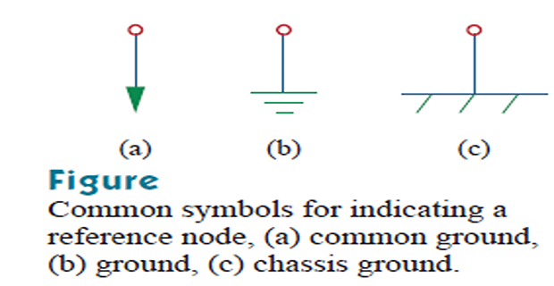
The reference node. Voltage is meaningful only between two points, so we begin by nominating one node as the reference or ground node and declaring its potential to be zero. Every other node voltage is then measured with respect to it. The choice is arbitrary in principle, but a sensible one saves work: pick the node with the most branches connected to it, which is usually the bottom rail, and if a voltage source is connected to ground, pick the node at its negative terminal so that the source directly fixes one unknown.
Select a reference node and assign it zero potential.
Assign voltages \(v_{1}, v_{2}, \ldots, v_{n-1}\) to the remaining \(n-1\) non-reference nodes.
Apply KCL at each non-reference node, expressing every branch current by Ohm's law in terms of the node voltages.
Solve the resulting \(n-1\) simultaneous equations.
The one step that causes trouble is the third, and a single rule removes the difficulty. For a resistor connecting node \(j\) to node \(k\), the current flowing from \(j\) to \(k\) is
Adopt the convention that current always leaves the node you are writing the equation for, and this reduces to a mechanical rule: at node \(j\), every resistor branch contributes \((v_j - v_{\text{other}})/R\), and the sum of these equals the total current injected into the node by sources. There is then no sign to think about at all.
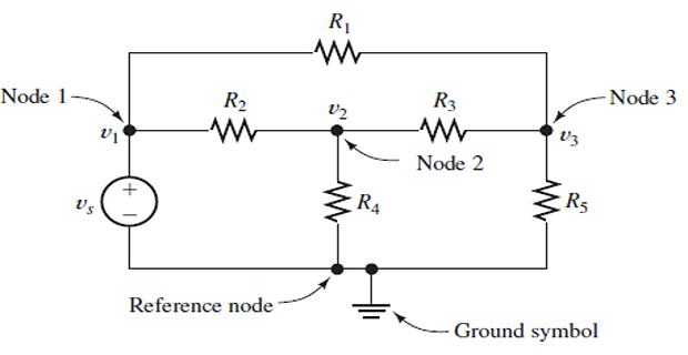
Problem. Determine the node voltages \(v_{1}\) and \(v_{2}\) in the circuit below, then find the current in the 3 \(\Omega\) resistor and verify the power balance.
Solution. Take the bottom rail as reference. There are three nodes, so \(n - 1 = 2\) equations are needed.
At node 1, currents leaving through the 4 \(\Omega\) and the 3 \(\Omega\) must equal the 5 A injected:
At node 2, current arrives from node 1 through the 3 \(\Omega\) and 1 A is injected; both leave through the 2 \(\Omega\):
Clearing fractions — multiply the first by 12 and the second by 6:
Solving the pair — multiply the first by 5, the second by 4, and add:
The current in the 3 \(\Omega\) resistor, flowing from node 1 to node 2, is
Power check. The 4 \(\Omega\) carries \(12/4 = 3\) A and the 2 \(\Omega\) carries \(6/2 = 3\) A:
Note that a current source's power requires the voltage across it, which is simply the node voltage it feeds — one of the incidental conveniences of having solved for node voltages in the first place.
Nodal Analysis with Voltage Sources
A voltage source appears to defeat nodal analysis, because we cannot write the current through it in terms of the node voltages — an ideal source supplies whatever current is required, and that current is unknown. Two cases arise, and only the second needs a new idea.
Case 1 — the source connects a node to the reference. Then the node voltage is simply known, equal to the source value, and no equation is needed for it at all. The unknown count drops by one, which is why choosing the reference at a grounded source's negative terminal is such a good move.
Case 2 — the source connects two non-reference nodes. This calls for the supernode. Enclose the source and its two nodes in a closed boundary, treating the whole region as a single generalised node. Recall from Section 2.5 that KCL applies to any closed boundary, not merely to a point — that generalisation is exactly what licenses this manoeuvre.
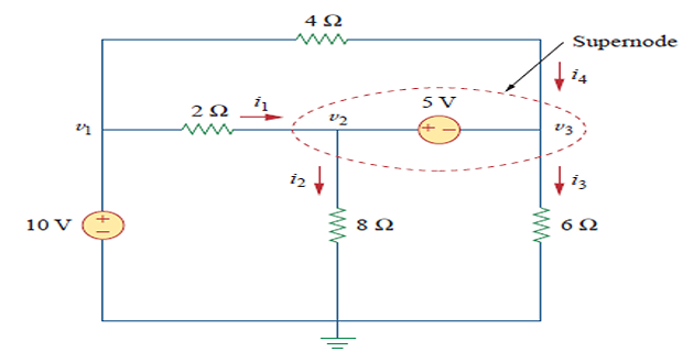
Two equations then replace the two that were lost:
KCL for the supernode — sum the currents in every branch that crosses the boundary, ignoring the source branch entirely since it lies inside.
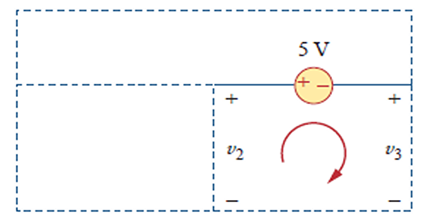
The constraint equation — the source itself fixes the difference between the two node voltages, \(v_{j} - v_{k} = V_{s}\), with the sign taken from the source polarity.
The count is unchanged: two nodes, two equations. Only their character has changed, one being a KCL statement and one an algebraic constraint.
Problem. Find \(v_{1}\) and \(v_{2}\) in the circuit below.
Solution. Apply KCL to the supernode. The branches crossing the dashed boundary are the 6 A source entering, and the 2 \(\Omega\) and 4 \(\Omega\) resistors leaving to ground. The 6 V source is inside and does not appear:
The constraint comes from the source, whose positive terminal is at node 1:
Substituting \(v_{1} = v_{2} + 6\) into the KCL equation:
Check. Substituting back, \(10/2 + 4/4 = 5 + 1 = 6\) A \(\checkmark\), and \(10 - 4 = 6\) V \(\checkmark\). The current delivered by the 6 V source is not needed to solve the circuit, but can be recovered afterwards by applying KCL at node 1 alone: \(6 = 10/2 + i_{s}\) gives \(i_{s} = 1\) A flowing from node 1 into the source.
Mesh Analysis
Mesh analysis is the exact dual of nodal analysis. Where nodal analysis applies KCL and solves for node voltages, mesh analysis applies KVL and solves for mesh currents.
A mesh is a loop that contains no other loop within it — a "window pane" of the circuit diagram. Mesh analysis applies only to planar circuits: those that can be drawn on a flat surface with no branches crossing. Most circuits of practical interest are planar, but not all, and for a non-planar circuit nodal analysis remains available while mesh analysis does not. This is the one genuine asymmetry between the two methods.
A mesh current is a fictitious current assumed to circulate around the perimeter of a mesh. It is not directly measurable. What is measurable is the branch current, which for a branch shared by two meshes is the difference of the two mesh currents. This is the essential bookkeeping trick: by construction, every mesh current enters and leaves each node it passes through, so KCL is satisfied automatically and only KVL remains to be imposed.
Assign mesh currents \(i_{1}, i_{2}, \ldots, i_{\ell}\) to the \(\ell\) meshes. Choose the same direction — conventionally clockwise — for all of them; this makes every mutual term negative and allows the by-inspection shortcut of Section 3.6.
Apply KVL around each mesh, expressing each resistor voltage by Ohm's law in terms of the mesh currents.
Solve the resulting \(\ell\) simultaneous equations.
The rule that removes all sign difficulty is this: for a resistor belonging to mesh \(j\) alone, the drop is \(R\,i_{j}\); for a resistor shared with mesh \(k\), the drop as seen from mesh \(j\) is \(R\left(i_{j} - i_{k}\right)\). The current of the mesh you are working in always comes first.
Problem. Find the mesh currents in the circuit below, and hence the current in the shared 4 \(\Omega\) resistor. Verify by a power balance.
Solution. There are two meshes, so two KVL equations are needed. Travelling clockwise and entering drops as positive:
Mesh 1 — the 20 V source is a rise, the 2 \(\Omega\) belongs to mesh 1 alone, and the 4 \(\Omega\) is shared:
Mesh 2 — the shared 4 \(\Omega\) now seen from mesh 2, then the 8 \(\Omega\), then the 4 V source as a drop:
From the second equation, \(i_{1} = 3i_{2} + 1\). Substituting into the first:
The current in the shared resistor, taken in the direction of \(i_1\), is
Power check.
The 4 V source absorbs, since \(i_2\) is driven through it against its polarity by the larger source — the charging-battery situation of Chapter 2 again.
Mesh Analysis with Current Sources
A current source is to mesh analysis what a voltage source is to nodal analysis: an obstacle, because the voltage across an ideal current source is unknown. Once again two cases arise.
Case 1 — the source belongs to one mesh only. Then that mesh current is simply known, equal to the source current (with sign set by direction), and no KVL equation is written for that mesh. One unknown disappears.
Case 2 — the source is shared between two meshes. This calls for the supermesh. Form a single larger loop by taking the two meshes together and excluding the branch containing the current source, then apply KVL around that combined path. Since the path avoids the source, its unknown voltage never enters the equation.
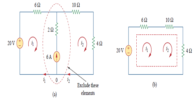
As with the supernode, two equations replace the two that were lost:
KVL around the supermesh, omitting the current-source branch.
The constraint equation supplied by the source itself, \(i_{j} - i_{k} = I_{s}\), with the sign set by the source direction relative to the assumed mesh currents.
The symmetry with Section 3.3 is exact and worth noticing: supernode is to voltage source as supermesh is to current source, and in both cases the trick is to route the analysis around the troublesome element and pick up the missing information from a constraint.
Problem. Find the mesh currents in the circuit below, and determine the voltage across the 3 A source.
Solution. Apply KVL around the outer loop, which passes through the 24 V source, the 2 \(\Omega\) and the 4 \(\Omega\) but avoids the current source entirely:
The constraint comes from the source. Its 3 A flows upward in the shared branch; taking both mesh currents clockwise, the shared branch carries \(i_{2} - i_{1}\) upward, so
Substituting \(i_{1} = i_{2} - 3\):
Voltage across the source. This was deliberately excluded from the supermesh equation, so recover it afterwards by applying KVL to mesh 1 alone. Let \(v_{s}\) be the drop across the source in the clockwise direction of \(i_1\):
Power check. The resistors absorb \((2)^2(2) = 8\) W and \((5)^2(4) = 100\) W, totalling 108 W. The 24 V source carries \(i_1 = 2\) A and supplies 48 W; the current source carries 3 A at 20 V and therefore supplies 60 W. The totals agree: \(48 + 60 = 108\) W \(\checkmark\).
This is the general pattern with both supernodes and supermeshes — the quantity you excluded to make the analysis possible is always recoverable at the end from a local application of the law you set aside.
Analysis by Inspection
Once you have written a few sets of equations by hand, a pattern becomes unmistakable, and the equations can be written straight down in matrix form without deriving them. This works whenever the circuit contains only independent sources, and it is by far the fastest route for hand analysis of a well-behaved network.
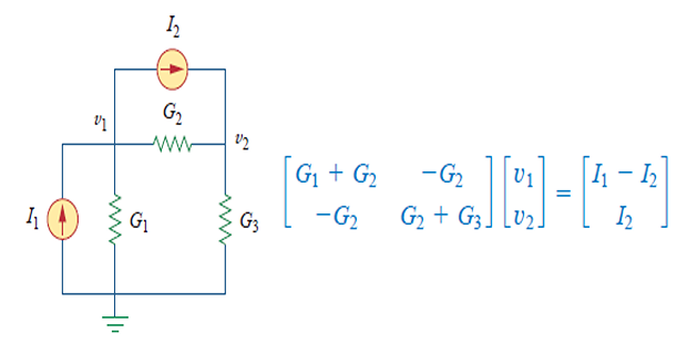
Nodal, by inspection. For a circuit with \(N\) non-reference nodes,
\(G_{kk}\) — the self-conductance: the sum of all conductances connected to node \(k\). Always positive.
\(G_{kj}\) for \(k \neq j\) — the mutual conductance: the negative of the sum of conductances directly joining nodes \(k\) and \(j\). Always negative or zero.
\(i_{k}\) — the net current injected into node \(k\) by sources.
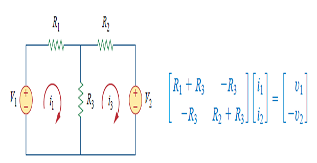
Mesh, by inspection. For a circuit with \(N\) meshes, all currents taken clockwise,
\(R_{kk}\) — the self-resistance: the sum of all resistances in mesh \(k\). Always positive.
\(R_{kj}\) for \(k \neq j\) — the mutual resistance: the negative of the sum of resistances shared by meshes \(k\) and \(j\). Negative provided all mesh currents circulate the same way.
\(v_{k}\) — the net voltage rise driving mesh \(k\) clockwise.
Both matrices are symmetric — \(G_{kj} = G_{jk}\) and \(R_{kj} = R_{jk}\). That symmetry is a consequence of reciprocity in networks of passive bilateral elements, and it is an excellent error check: if your matrix is not symmetric, you have made a mistake. Note that dependent sources destroy the symmetry, which is precisely why the by-inspection method is restricted to independent sources.
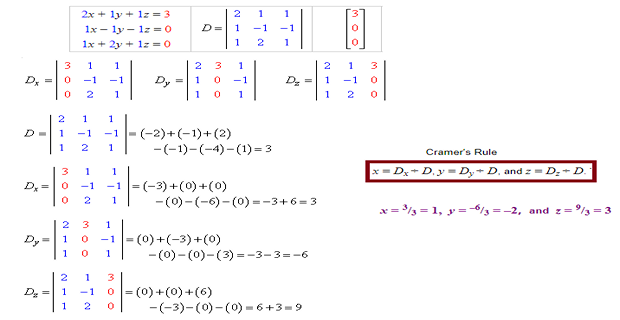
Problem. Write the nodal equations for the circuit of Example 3.1 and the mesh equations for the circuit of Example 3.3, by inspection, and solve each by Cramer's rule.
Nodal (Example 3.1 circuit). Node 1 has the 4 \(\Omega\) to ground and the 3 \(\Omega\) to node 2; node 2 has the 3 \(\Omega\) to node 1 and the 2 \(\Omega\) to ground:
The determinant and the two solutions:
Identical to the answers obtained the long way in Example 3.1 \(\checkmark\).
Mesh (Example 3.3 circuit). Mesh 1 contains 2 \(\Omega\) and 4 \(\Omega\); mesh 2 contains 4 \(\Omega\) and 8 \(\Omega\); they share the 4 \(\Omega\). The 20 V source drives mesh 1 clockwise, the 4 V source opposes mesh 2:
Again identical to Example 3.3 \(\checkmark\). Both matrices came out symmetric, as they must. Notice how much less work this was than deriving the equations from scratch — for a three- or four-mesh circuit the saving is considerable.
Nodal versus Mesh: Which to Choose
Both methods always work on a planar circuit and always give the same answer. The choice is purely one of economy, and three considerations settle it.
| Consideration | Favours nodal | Favours mesh |
|---|---|---|
| Number of equations | fewer nodes than meshes | fewer meshes than nodes |
| Source types present | mostly current sources | mostly voltage sources |
| Quantity actually required | node or element voltages | branch currents |
| Circuit is non-planar | the only option | not applicable |
| Parallel-connected elements | natural fit | awkward |
| Series-connected elements | awkward | natural fit |
The equation count is the first thing to check, and it is settled by the topology relation of Section 2.4. A circuit with \(n\) nodes and \(b\) branches needs \(n-1\) nodal equations or \(b-n+1\) mesh equations; simply compute both and take the smaller.
The second consideration reflects what each method finds awkward. A voltage source forces a supernode in nodal analysis but is trivially handled in mesh analysis; a current source forces a supermesh in mesh analysis but is trivially handled in nodal analysis. A circuit driven entirely by current sources into a set of parallel branches is a nodal problem; a single loop with several series voltage sources is a mesh problem.
The third is easily overlooked. If a problem asks only for the voltage across one element, nodal analysis may deliver it immediately while mesh analysis requires a further step. Solve for what you were asked for.
When both are equally convenient, doing the problem both ways is the most reliable check available — an error in one method almost never reproduces itself in the other.
Circuits with Dependent Sources
Dependent sources, introduced in Section 1.6, require no new method — only one extra step. Treat the dependent source exactly as though it were independent while writing the KCL or KVL equations, then add a constraint equation expressing the controlling variable in terms of the chosen unknowns.
Because the controlling variable must be expressed in node voltages (for nodal) or mesh currents (for mesh), the constraint eliminates one variable and the system closes. Two points are worth stating plainly:
A dependent source is never deactivated or ignored, no matter what the technique. It remains active at all times.
The resulting matrix is generally not symmetric, so the by-inspection method of Section 3.6 does not apply. Write the equations out.
Problem. In a two-node circuit, a 3 A independent source feeds node 1. Node 1 connects to ground through 4 \(\Omega\) and to node 2 through 2 \(\Omega\). Node 2 connects to ground through 6 \(\Omega\) and is also fed by a dependent current source of value \(2i_{x}\), where \(i_{x}\) is the current flowing from node 1 to node 2 through the 2 \(\Omega\) resistor. Find \(v_{1}\), \(v_{2}\) and \(i_{x}\).
Solution. The constraint is written first, since everything else depends on it:
At node 1:
At node 2, the current arriving through the 2 \(\Omega\) plus the dependent source current must leave through the 6 \(\Omega\):
Substituting the constraint into the node-2 equation removes \(i_x\):
Now use the node-1 equation. Multiplying through by 4:
Check. Node 1: \(10/4 + 0.5 = 2.5 + 0.5 = 3\) A \(\checkmark\). Node 2: \(0.5 + 2(0.5) = 1.5\) A entering, and \(9/6 = 1.5\) A leaving \(\checkmark\). Note that the dependent source here delivers 1 A into node 2 — twice the 0.5 A flowing through the controlling resistor — which is exactly the amplifying behaviour that makes dependent sources the model for transistors.
Application: DC Transistor Bias Circuits
The most important application of this chapter is one you will meet again in every electronics course. A bipolar junction transistor, for DC purposes, is a two-port device described by two simple relations, and once those are written down the surrounding circuit is nothing more than a resistive network with a dependent source in it — exactly the situation of Section 3.8.
For an npn transistor operating in the active region, the two relations are
where \(\beta\) is the common-emitter current gain, typically between 50 and 300. The second relation is nothing but KCL applied to the transistor as a node. In addition, the base–emitter junction behaves as a forward-biased diode, so to a good approximation
These three statements, together with KVL round the base loop and the collector loop, determine the operating point completely. The purpose of the bias network is to place that operating point where the transistor amplifies faithfully — neither cut off nor saturated.
Problem. A common-emitter stage has \(V_{CC} = 12~\mathrm{V}\), a base resistor \(R_{B} = 100~\mathrm{k}\Omega\) from the supply to the base, and a collector resistor \(R_{C} = 500~\Omega\). Taking \(\beta = 100\) and \(V_{BE} = 0.7~\mathrm{V}\), find \(I_{B}\), \(I_{C}\), \(I_{E}\) and the collector voltage \(V_{C}\).
Solution. KVL around the base loop, from the supply through \(R_B\) and the base–emitter junction to ground:
The collector current follows from the current gain, and the emitter current from KCL:
Finally KVL around the collector loop:
The collector sits at 6.35 V, roughly half the supply — a healthy operating point, leaving room for the output to swing in both directions without clipping.
A design warning worth absorbing. This fixed-bias arrangement is analytically simple and practically poor. Since \(I_C = \beta I_B\) and \(I_B\) is fixed by \(R_B\) alone, the operating point is directly proportional to \(\beta\) — a parameter that varies by a factor of three between nominally identical devices and drifts substantially with temperature. Replacing the transistor could push this stage into saturation. Practical designs use an emitter resistor to provide negative feedback, which you will analyse with exactly the methods of this chapter.
Summary and Key Formulas
Nodal analysis applies KCL at each of the \(n-1\) non-reference nodes, with node voltages as unknowns.
A voltage source between two non-reference nodes requires a supernode: KCL across the enclosing boundary, plus the constraint \(v_j - v_k = V_s\).
Mesh analysis applies KVL around each of the \(\ell = b - n + 1\) meshes, with mesh currents as unknowns. It requires a planar circuit.
A current source shared by two meshes requires a supermesh: KVL around the combined loop excluding the source, plus the constraint \(i_j - i_k = I_s\).
With only independent sources present, both the conductance matrix \(\mathbf{G}\) and the resistance matrix \(\mathbf{R}\) can be written by inspection, and both are symmetric.
Choose the method giving fewer equations, matching the source types present and the quantity actually required.
Dependent sources are treated as ordinary sources plus one constraint equation, and they destroy matrix symmetry.
A DC transistor bias circuit is a resistive network with a dependent source, governed by \(I_C = \beta I_B\), \(I_E = (1+\beta)I_B\) and \(V_{BE} \approx 0.7\) V.
| Result | Formula | Notes |
|---|---|---|
| Number of nodal equations | \(n-1\) | \(n\) = total nodes |
| Number of mesh equations | \(\ell = b-n+1\) | planar circuits only |
| Branch current, nodal | \(i = \dfrac{v_j - v_k}{R}\) | from node \(j\) to node \(k\) |
| Shared-branch current, mesh | \(i = i_j - i_k\) | own mesh current first |
| Supernode constraint | \(v_j - v_k = V_s\) | plus KCL across the boundary |
| Supermesh constraint | \(i_j - i_k = I_s\) | plus KVL round the outer loop |
| Nodal matrix form | \(\mathbf{G}\mathbf{v} = \mathbf{i}\) | \(G_{kk}>0\), \(G_{kj}\le 0\), symmetric |
| Mesh matrix form | \(\mathbf{R}\mathbf{i} = \mathbf{v}\) | \(R_{kk}>0\), \(R_{kj}\le 0\), symmetric |
| Cramer's rule, \(2\times2\) | \(x_1 = \dfrac{b_1a_{22}-a_{12}b_2}{a_{11}a_{22}-a_{12}a_{21}}\) | practical to three unknowns |
| Transistor collector current | \(I_C = \beta I_B\) | active region |
| Transistor emitter current | \(I_E = (1+\beta)I_B\) | KCL at the device |
| Base–emitter drop | \(V_{BE} \approx 0.7~\mathrm{V}\) | silicon, forward biased |
Common Mistakes
Writing a KCL equation for a node whose voltage is already known. If a voltage source connects a node to ground, that node voltage is fixed. Writing an equation for it introduces the source's unknown current and wastes the advantage.
Including the source branch in a supernode KCL equation. The source is inside the boundary; only branches crossing the boundary contribute.
Forgetting the constraint equation. A supernode or supermesh always needs two equations, not one. Writing only the KCL or KVL statement leaves the system underdetermined.
Including the current-source branch in a supermesh KVL. The whole point is to route around it. Its voltage is unknown and must not appear.
Mixing mesh-current directions. Choosing some clockwise and some anticlockwise is legal but makes mutual terms positive and breaks the by-inspection rule. Keep them all clockwise.
Reversing the order in a shared-branch term. From mesh \(j\) the drop is \(R(i_j - i_k)\), not \(R(i_k - i_j)\). Your own mesh current comes first, always.
Using the by-inspection method when a dependent source is present. The matrix is no longer symmetric and the rules give wrong entries. Write the equations out.
Deactivating a dependent source. It is never suppressed, in this chapter or in Chapter 4's theorems.
Attempting mesh analysis on a non-planar circuit. If branches must cross, meshes are undefined. Use nodal analysis.
Not checking the matrix for symmetry. With independent sources only, an asymmetric matrix is a guaranteed sign that something is wrong — a free check you should always take.
Chapter Review
Work these before opening the answers. Use a power balance as a check wherever a circuit is fully solved.
P3.1 A 3 A source feeds node 1, which connects to ground through 6 \(\Omega\) and to node 2 through 4 \(\Omega\). Node 2 connects to ground through 8 \(\Omega\). Find \(v_1\) and \(v_2\).
Show answer
Node 1: \(3 = \frac{v_1}{6} + \frac{v_1-v_2}{4}\). Node 2: \(\frac{v_1-v_2}{4} = \frac{v_2}{8}\), giving \(2(v_1-v_2) = v_2\) so \(v_1 = 1.5v_2\).\[3 = \frac{1.5v_2}{6} + \frac{0.5v_2}{4} = 0.25v_2 + 0.125v_2 = 0.375v_2\]\[v_2 = 8~\mathrm{V}, \qquad v_1 = 12~\mathrm{V}\]P3.2 Two meshes share a 6 \(\Omega\) resistor. Mesh 1 contains an 18 V source and a 2 \(\Omega\); mesh 2 contains a 6 \(\Omega\) and a 6 V source that opposes \(i_2\). Find both mesh currents and the power supplied by the 18 V source.
Show answer
\[-18 + 2i_1 + 6(i_1-i_2) = 0 \;\Rightarrow\; 8i_1 - 6i_2 = 18\]Solving: \(i_1 = 3~\mathrm{A}\), \(i_2 = 1~\mathrm{A}\). The source supplies \((18)(3) = 54\) W. Check: \(2\Omega\) absorbs 18 W, shared \(6\Omega\) absorbs \((2)^2(6)=24\) W, mesh-2 \(6\Omega\) absorbs 6 W, and the 6 V source absorbs 6 W — total 54 W \(\checkmark\).\[6(i_2-i_1) + 6i_2 + 6 = 0 \;\Rightarrow\; -6i_1 + 12i_2 = -6\]P3.3 An 8 A source feeds node 1, which connects to ground through 2 \(\Omega\). An 8 V source with its positive terminal at node 1 joins node 1 to node 2, and node 2 connects to ground through 6 \(\Omega\). Find \(v_1\) and \(v_2\).
Show answer
Supernode KCL and constraint:\[8 = \frac{v_1}{2} + \frac{v_2}{6}, \qquad v_1 - v_2 = 8\]Check: \(14/2 + 6/6 = 7 + 1 = 8\) A \(\checkmark\).\[8 = \frac{v_2+8}{2} + \frac{v_2}{6} = \frac{2v_2}{3} + 4 \;\Rightarrow\; v_2 = 6~\mathrm{V}, \quad v_1 = 14~\mathrm{V}\]P3.4 Two meshes share a branch containing a 3 A source directed so that \(i_2 - i_1 = 3\). The outer loop contains a 30 V source, a 2 \(\Omega\) in mesh 1 and a 4 \(\Omega\) in mesh 2. Find both mesh currents.
Show answer
\[-30 + 2i_1 + 4i_2 = 0, \qquad i_2 - i_1 = 3\]\[2(i_2-3) + 4i_2 = 30 \;\Rightarrow\; 6i_2 = 36 \;\Rightarrow\; i_2 = 6~\mathrm{A}, \quad i_1 = 3~\mathrm{A}\]P3.5 A planar network has 9 branches and 6 nodes. How many equations does each method require, and which would you choose?
Show answer
Nodal: \(n - 1 = 5\) equations. Mesh: \(\ell = b - n + 1 = 9 - 6 + 1 = 4\) equations. Mesh analysis is more economical — though if the network is driven mainly by current sources, the supermeshes it would force could easily cancel that advantage.P3.6 Write the conductance matrix by inspection for a three-node circuit in which node 1 has 1 \(\Omega\) to ground and 2 \(\Omega\) to node 2; node 2 has 4 \(\Omega\) to node 3; node 3 has 5 \(\Omega\) to ground.
Show answer
The zero entries record that nodes 1 and 3 are not directly connected. The matrix is symmetric, as expected.\[\mathbf{G} = \begin{bmatrix} 1+\tfrac{1}{2} & -\tfrac{1}{2} & 0 \\[3pt] -\tfrac{1}{2} & \tfrac{1}{2}+\tfrac{1}{4} & -\tfrac{1}{4} \\[3pt] 0 & -\tfrac{1}{4} & \tfrac{1}{4}+\tfrac{1}{5}\end{bmatrix} = \begin{bmatrix} 1.5 & -0.5 & 0 \\ -0.5 & 0.75 & -0.25 \\ 0 & -0.25 & 0.45 \end{bmatrix}\]P3.7 In Worked Example 3.6, what would \(v_2\) become if the dependent source were removed altogether?
Show answer
Node 2 becomes \(\frac{v_1-v_2}{2} = \frac{v_2}{6}\), so \(3(v_1-v_2) = v_2\) and \(v_1 = \frac{4}{3}v_2\). Node 1 gives \(12 = 3v_1 - 2v_2 = 4v_2 - 2v_2 = 2v_2\), so \(v_2 = 6~\mathrm{V}\) and \(v_1 = 8~\mathrm{V}\). The dependent source raised \(v_2\) from 6 V to 9 V — a 50 % increase, which is the amplification it provides.P3.8 For the circuit of Worked Example 3.1, verify the answers by mesh analysis instead. (Hint: both sources are current sources, so each fixes a mesh current directly.)
Show answer
With three meshes and two current sources each in a single mesh, two mesh currents are known immediately and only one KVL equation remains. The branch currents come out as 3 A in the 4 \(\Omega\), 2 A in the 3 \(\Omega\) and 3 A in the 2 \(\Omega\), giving \(v_1 = 3\times4 = 12\) V and \(v_2 = 3\times2 = 6\) V \(\checkmark\). Nodal was the better choice here — two equations rather than three meshes to set up.P3.9 A fixed-bias stage has \(V_{CC} = 15~\mathrm{V}\), \(R_B = 220~\mathrm{k}\Omega\), \(R_C = 1~\mathrm{k}\Omega\), \(\beta = 120\) and \(V_{BE} = 0.7~\mathrm{V}\). Find \(I_B\), \(I_C\) and \(V_C\).
Show answer
\[I_B = \frac{15-0.7}{220\times10^{3}} = \frac{14.3}{220\,000} = 65.00~\mu\mathrm{A}\]\[I_C = 120(65.00\times10^{-6}) = 7.800~\mathrm{mA}\]\[V_C = 15 - (7.800\times10^{-3})(1000) = 15 - 7.800 = 7.200~\mathrm{V}\]P3.10 A circuit contains four voltage sources, no current sources, 5 nodes and 8 branches. Which method would you use, and why?
Show answer
Mesh analysis. The counts are close — nodal needs 4 equations, mesh needs \(8-5+1 = 4\) — but with four voltage sources and no current sources, nodal analysis risks several supernodes while mesh analysis handles every voltage source trivially as a term in the KVL sum. Source type decides it when the equation counts tie.
MCQ 1. Nodal analysis is the systematic application of:
(a) Ohm's law (b) KCL (c) KVL (d) superpositionShow answer
(b) KCL. Mesh analysis is the systematic application of KVL.MCQ 2. A circuit has 6 nodes. The number of nodal equations required is:
(a) 4 (b) 5 (c) 6 (d) 7Show answer
(b) 5. One node is the reference, leaving \(n-1 = 5\).MCQ 3. A supernode is required when a voltage source is connected between:
(a) a node and ground (b) two non-reference nodes (c) two meshes (d) two branches in seriesShow answer
(b) two non-reference nodes. A source to ground simply fixes that node voltage and needs no special treatment.MCQ 4. Mesh analysis can be applied only to circuits that are:
(a) linear (b) planar (c) passive (d) balancedShow answer
(b) planar. Meshes are undefined if branches must cross; nodal analysis has no such restriction.MCQ 5. In a supermesh, KVL is written:
(a) including the current-source branch (b) excluding the current-source branch (c) only for the smaller mesh (d) twiceShow answer
(b) excluding it. The voltage across the source is unknown, so the path must avoid it.MCQ 6. In the conductance matrix written by inspection, the off-diagonal terms are:
(a) always positive (b) always negative or zero (c) always zero (d) of either signShow answer
(b) negative or zero — zero when the two nodes are not directly connected, negative otherwise.MCQ 7. A network has 10 branches and 7 nodes. The number of mesh equations is:
(a) 3 (b) 4 (c) 6 (d) 17Show answer
(b) 4. \(\ell = b - n + 1 = 10 - 7 + 1 = 4\).MCQ 8. When a circuit contains a dependent source, the by-inspection method fails because the matrix is no longer:
(a) square (b) symmetric (c) invertible (d) realShow answer
(b) symmetric. Symmetry depends on reciprocity, which dependent sources violate.MCQ 9. For a shared resistor, the voltage drop written in the equation for mesh 1 is:
(a) \(R(i_2-i_1)\) (b) \(R(i_1-i_2)\) (c) \(R(i_1+i_2)\) (d) \(Ri_1\)Show answer
(b) \(R(i_1-i_2)\). The mesh current you are writing for always comes first.MCQ 10. For a transistor in the active region with \(\beta = 100\) and \(I_B = 20~\mu\mathrm{A}\), the emitter current is:
(a) 2.00 mA (b) 2.02 mA (c) 1.98 mA (d) 20 \(\mu\)AShow answer
(b) 2.02 mA. \(I_E = (1+\beta)I_B = 101 \times 20~\mu\mathrm{A} = 2.02\) mA. Option (a) is \(I_C\), a tempting but incorrect answer.
Mesh analysis satisfies KCL automatically and imposes only KVL. Explain why, and identify the corresponding statement for nodal analysis.
Why is a mesh current described as fictitious when a branch current is not? In what sense can a mesh current still be said to exist?
The supernode and the supermesh are described in this chapter as duals. Set out the correspondence term by term, and say what plays the role of "ground" in the mesh world.
Why does the choice of reference node not affect any element voltage, and what practical difference does a good choice make?
Explain why the conductance and resistance matrices are symmetric for circuits of passive bilateral elements, and why a dependent source destroys that symmetry.
A colleague solves a circuit by nodal analysis and gets a different answer from yours by mesh analysis. Neither of you can find an arithmetic error. What structural mistakes should you check for first?
Nodal and mesh analysis are complete methods: given any linear circuit, they will produce the answer. But they are also indiscriminate — they solve for everything, even when you want one current in one branch, and they must be redone from scratch every time a single element value changes.
Chapter 4 takes a different approach. Linearity, superposition, source transformation and above all Thévenin's and Norton's theorems let you replace an entire complicated network by a single source and a single resistance, as seen from the terminals you care about. When you need to know how one load responds to a whole network — and how it responds as the load is varied — that reduction is worth far more than another set of simultaneous equations.