By the end of this chapter you should be able to:
State the linearity property and use proportionality to solve ladder networks by assumption.
Apply the superposition theorem, deactivating independent sources correctly while leaving dependent sources active.
Convert freely between a voltage source in series with a resistance and a current source in parallel with it.
Find the Thévenin and Norton equivalents of any linear network at a chosen pair of terminals.
Determine \(R_{Th}\) by the test-source method when dependent sources are present.
State and derive the maximum power transfer condition and compute the maximum power delivered.
Model a practical source by its open-circuit voltage and internal resistance.
Analyse a Wheatstone bridge at balance and use it to measure an unknown resistance.
Introduction
Nodal and mesh analysis will solve any linear circuit, but they are blunt instruments. They compute everything when you may want one quantity, and they must be repeated from scratch whenever a single element value changes. If you are designing a loudspeaker to be driven by an amplifier, or choosing a load resistor to extract the most power from a sensor, what you actually want is a compact description of the network as seen from two terminals — one that stays valid as the load varies.
That is what this chapter provides. Every result here rests on one property, linearity, which is why none of them apply to circuits containing non-linear elements. From linearity flow superposition and source transformation, and from those in turn flow Thévenin's and Norton's theorems — arguably the two most useful results in all of circuit analysis. Maximum power transfer is then an immediate corollary.
The theorems are labour-saving devices, not new physics. Anything they tell you could in principle be extracted from Chapter 3's methods. What they add is insight: the knowledge that an arbitrarily complicated network behaves at its terminals exactly like one source and one resistor is a genuinely powerful idea, and it recurs throughout the rest of this book — in the frequency domain in Chapter 10, and again in two-port form in Chapter 19.
The Linearity Property
A circuit is linear if it contains only linear elements, linear dependent sources and independent sources. Linearity has two components, and it is worth separating them because they are used differently.
Homogeneity (scaling). If the input is multiplied by a constant, the response is multiplied by the same constant. For a resistor, \(v = iR\) gives \(kv = (ki)R\).
Additivity. The response to a sum of inputs is the sum of the responses to each input applied alone. If \(v_1 = i_1R\) and \(v_2 = i_2R\), then \(\left(i_1+i_2\right)R = v_1 + v_2\).
Additivity is exactly the superposition theorem of the next section. Homogeneity gives us something else — a technique for ladder networks.
An important caution about power. Power is not a linear function of the source. Since \(p = i^{2}R\), doubling the source current quadruples the power. This is why superposition can never be applied to power, a point Section 4.3 returns to and one that costs students marks every year.
Problem. A ladder network is driven by a source \(V_{s}\) through a 2 \(\Omega\) series resistor. At the first node a 3 \(\Omega\) resistor goes to ground; a 2 \(\Omega\) resistor continues to a second node, where a 4 \(\Omega\) resistor goes to ground. Find the current \(i_{o}\) in the 4 \(\Omega\) resistor when \(V_{s} = 30~\mathrm{V}\).
Solution. Rather than working forwards, assume the answer and work backwards to find the source it implies. Take \(i_{o} = 1~\mathrm{A}\). Then
The same 1 A flows through the second 2 \(\Omega\) resistor, so
The 3 \(\Omega\) shunt therefore carries \(6/3 = 2\) A, and by KCL the source branch carries
So an assumed output of 1 A corresponds to a source of 12 V. By homogeneity, the actual 30 V source scales everything by the same factor:
Check by direct reduction. Working from the far end, \(2 + 4 = 6~\Omega\), in parallel with 3 \(\Omega\) gives 2 \(\Omega\), plus the series 2 \(\Omega\) gives \(R_{eq} = 4~\Omega\). Then \(i_s = 30/4 = 7.5\) A, \(v_1 = 30 - 7.5(2) = 15\) V, and \(i_o = 15/6 = 2.5\) A \(\checkmark\).
The assumption method comes into its own for longer ladders, where each backward step is a single multiplication or addition while the forward reduction requires repeated parallel combinations.
Superposition
The superposition theorem states that in a linear circuit with more than one independent source, the voltage across (or current through) any element is the algebraic sum of the voltages (or currents) produced by each independent source acting alone.
To apply it, consider the sources one at a time and deactivate all the others. Deactivation means setting a source's value to zero, and what that implies depends on the type of source.
The last point cannot be over-emphasised. A dependent source is not an independent input to the circuit — it is part of the circuit's internal behaviour, like a resistor. It remains active in every sub-circuit, and its controlling variable must be recomputed for each one.
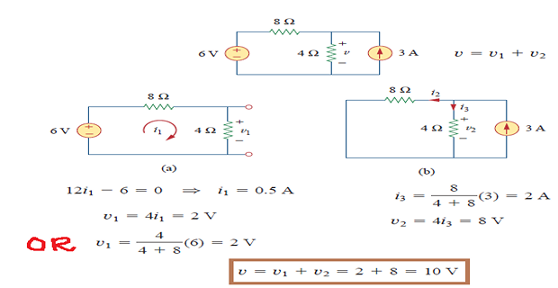
When is superposition worth using? Honestly, for a two-source circuit it is often slower than nodal analysis, because you solve two circuits instead of one. Its real value is conceptual and appears later: it is what allows a circuit's response to be split into a DC bias term and an AC signal term, and it underlies the whole of frequency-domain analysis, where sources at different frequencies must be treated separately.
Problem. A 24 V source in series with an 8 \(\Omega\) resistor feeds a node. An 8 \(\Omega\) resistor connects that node to ground, and a 4 A current source injects into the node. Find the node voltage \(v\) by superposition.
Solution, part 1 — the 24 V source acting alone. Deactivate the 4 A source by replacing it with an open circuit. The circuit becomes a simple voltage divider between the two 8 \(\Omega\) resistors:
Part 2 — the 4 A source acting alone. Deactivate the 24 V source by replacing it with a short circuit. The two 8 \(\Omega\) resistors are now in parallel, and the 4 A flows through the combination:
Sum.
Check by nodal analysis. Writing KCL at the node directly:
And a warning. The power in the 8 \(\Omega\) shunt resistor is \(28^{2}/8 = 98\) W. Superposing the partial powers would give \(12^{2}/8 + 16^{2}/8 = 18 + 32 = 50\) W — badly wrong. Superpose voltages and currents, then compute power once, at the end.
Problem. A single loop contains, in order: a 30 V source, a 4 \(\Omega\) resistor, a current-controlled voltage source of value \(2i\) (a drop in the direction of \(i\)), a 2 \(\Omega\) resistor, and a 6 V source opposing the 30 V source. Find \(i\) by superposition.
Solution, part 1 — the 30 V source alone. Short the 6 V source, but keep the dependent source:
Part 2 — the 6 V source alone. Short the 30 V source, again keeping the dependent source:
Sum.
Check by direct KVL on the original circuit:
Notice that the dependent source contributed its \(2i\) term to both sub-circuits, with a different value of the controlling current in each. Had it been deactivated along with the independent sources, the sub-circuit equations would have read \(6i' = 30\) and \(6i'' = -6\), giving \(i = 5 - 1 = 4\) A — wrong by a third.
Source Transformation
A practical voltage source is a voltage source in series with a resistance; a practical current source is a current source in parallel with a resistance. These two are indistinguishable from outside their terminals, provided the values are correctly related, and either may be substituted for the other at any point in an analysis.
To see why, compute the open-circuit voltage and short-circuit current of each. For the series form, \(v_{oc} = v_{s}\) and \(i_{sc} = v_{s}/R\). For the parallel form, \(v_{oc} = i_{s}R\) and \(i_{sc} = i_{s}\). Matching both requires
with the resistance unchanged. Since a linear two-terminal network is completely characterised by any two of open-circuit voltage, short-circuit current and terminal resistance, matching two of them matches the third and the equivalence is exact.

Two points of practice:
Direction matters. The current-source arrow must point towards the terminal that was the positive terminal of the voltage source. Getting this backwards inverts the sign of everything downstream.
An ideal source cannot be transformed. An ideal voltage source has no series resistance, so the equivalent current would be infinite; an ideal current source has no parallel resistance. The transformation requires a finite, non-zero \(R\).

Problem. A 12 V source in series with 4 \(\Omega\) feeds a node; a 12 \(\Omega\) resistor connects the node to ground, and a 2 A source injects into the node. Find the node voltage \(v\).
Solution. Transform the 12 V source and its 4 \(\Omega\) series resistor into a current source in parallel with the same 4 \(\Omega\):
Now both sources are current sources feeding the same node, so they add, and both resistors are in parallel:
Check by nodal analysis on the original circuit:
The transformed route required no simultaneous equations at all — just an addition and a parallel combination. This is typical: source transformation shines when it lets you merge sources that were previously of different types.
Thévenin's Theorem
Thévenin's theorem states that any linear two-terminal network can be replaced, as far as anything connected to those terminals is concerned, by a voltage source \(V_{Th}\) in series with a resistance \(R_{Th}\), where
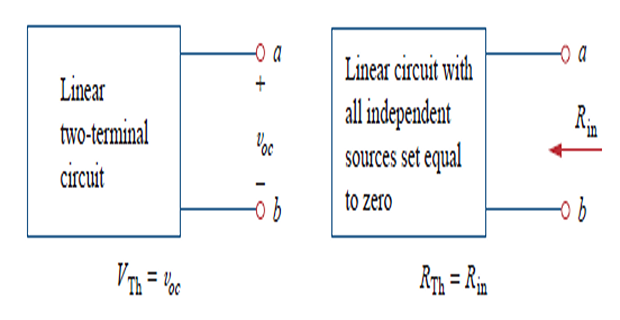
\(V_{Th}\) is the open-circuit voltage at the terminals — the voltage that appears when nothing is connected.
\(R_{Th}\) is the resistance seen looking back into the terminals with all independent sources deactivated.
The theorem's importance is hard to overstate. It says that a network of a thousand elements presents itself to the outside world as two numbers. If you then vary the load, you re-solve a two-element circuit rather than the whole network — which is exactly the situation in amplifier design, transducer interfacing and power distribution.
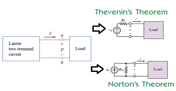
Why it works. The argument is superposition. Attach a current source of value \(i\) to the terminals and ask what terminal voltage results. By superposition the answer has two parts: the contribution of the network's own internal sources with \(i = 0\), which is \(V_{Th}\) by definition, plus the contribution of \(i\) with the internal independent sources deactivated, which is \(-iR_{Th}\). Hence
which is precisely the terminal relation of a voltage source in series with a resistance. No assumption was made about what is inside the network beyond linearity.
Remove the load from the terminals \(a\)–\(b\), leaving them open.
Find \(V_{Th}\) as the open-circuit voltage, by any method — nodal, mesh, division, transformation.
Find \(R_{Th}\). If the network contains only independent sources, deactivate them all (voltage sources shorted, current sources opened) and reduce the resulting resistive network by series and parallel combination. If dependent sources are present, use the methods of Section 4.7.
Reconnect the load across the equivalent and solve the simple two-element circuit.
Problem. Find the Thévenin equivalent of the network below at terminals \(a\)–\(b\). Then determine the current delivered to a 4 \(\Omega\) load.
Step 1 — \(V_{Th}\). With the terminals open, no current leaves at \(a\). Writing KCL at node \(A\), whose voltage equals \(V_{Th}\):
Multiplying through by 12:
Step 2 — \(R_{Th}\). Deactivate both independent sources: short the 24 V source and open the 3 A source. Looking in at \(a\)–\(b\), the 6 \(\Omega\) and 12 \(\Omega\) are then in parallel:
Step 3 — the load. With a 4 \(\Omega\) load across the equivalent,
Two elements replaced a four-element network, and if the load now changes to 10 \(\Omega\) the new current follows immediately as \(28/14 = 2\) A — no re-analysis required. That is the whole point of the theorem.
Norton's Theorem
Norton's theorem states that any linear two-terminal network can be replaced by a current source \(I_{N}\) in parallel with a resistance \(R_{N}\), where \(I_{N}\) is the short-circuit current at the terminals and \(R_{N}\) is the same resistance as \(R_{Th}\).
Norton's theorem is not an independent result — it is Thévenin's theorem plus one source transformation. The two equivalents are related by
This relation gives a valuable third route to \(R_{Th}\). Find any two of the three quantities and the third follows:
This is often the most reliable method, because it never requires you to decide what "looking into the terminals" means — you simply solve the network twice, once open and once shorted. It is also the only practical approach on a real piece of equipment, where you cannot reach inside to deactivate the sources.
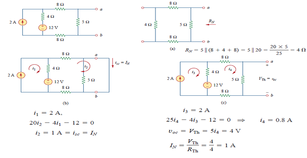
Problem. Find the Norton equivalent of the network of Example 4.5, computing \(I_{N}\) directly, and confirm consistency with the Thévenin result.
Solution. Short terminals \(a\)–\(b\). Node \(A\) is then held at 0 V, so no current flows in the 12 \(\Omega\) resistor — it is short-circuited. The entire short-circuit current is therefore whatever the two sources push through:
The Norton resistance equals the Thévenin resistance already found, \(R_{N} = 4~\Omega\). Checking consistency:
exactly the open-circuit voltage computed in Example 4.5. Equivalently, \(R_{Th} = v_{oc}/i_{sc} = 28/7 = 4~\Omega\), confirming the resistance by a third independent route.
Note how much easier \(I_{N}\) was than \(V_{Th}\) for this particular network — the short circuit removed a resistor from consideration entirely. Which of the two is easier depends on the topology, so it is worth glancing at both before committing.
Thévenin Resistance with Dependent Sources
When a network contains dependent sources, the "deactivate and reduce" method fails, because the dependent sources cannot be deactivated and so no purely resistive network remains to reduce. Two alternatives are available, and both give the same answer.
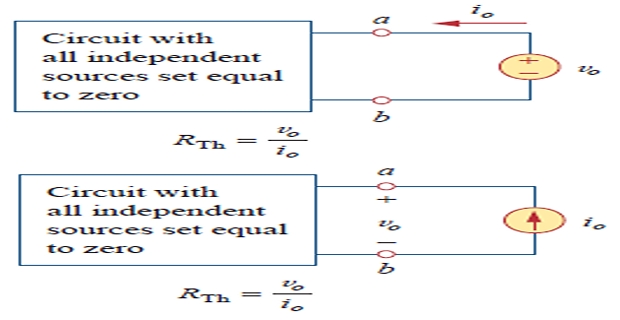
The open-circuit / short-circuit method. Compute \(v_{oc}\) and \(i_{sc}\) separately and take the ratio, \(R_{Th} = v_{oc}/i_{sc}\). This always works, but requires solving the network twice.
The test-source method. Deactivate the independent sources only, then apply a test source at the terminals — conventionally 1 V, or 1 A — and compute the resulting current or voltage. Then \(R_{Th} = v_{test}/i_{test}\).
The test-source method is usually faster and is the standard technique. Use a 1 V test source when the terminal voltage appears in the controlling expressions, and a 1 A test source when the terminal current does; either choice is legitimate.
A striking consequence worth noting: with dependent sources present, \(R_{Th}\) can be far larger than any resistance in the network, and it can even be negative. A negative \(R_{Th}\) is not an error — it signals a network capable of delivering power to any passive load, which is exactly the mechanism behind oscillators and negative-resistance amplifiers.
Problem. A network has terminals \(a\)–\(b\). From \(a\), a 4 \(\Omega\) resistor leads to an internal node \(c\); from \(c\), a 12 \(\Omega\) resistor returns to \(b\). A dependent current source of value \(2i_{x}\) drives current from \(b\) into node \(c\), where \(i_{x}\) is the current flowing from \(a\) to \(c\) through the 4 \(\Omega\). A 6 A independent source also injects into node \(c\). Find the Thévenin equivalent at \(a\)–\(b\).
Step 1 — \(R_{Th}\) by the test-source method. Deactivate the 6 A independent source (open circuit), keep the dependent source, and apply a 1 V test source at \(a\)–\(b\) with \(b\) as reference. Then \(v_{a} = 1~\mathrm{V}\) and
KCL at node \(c\): current arriving through the 4 \(\Omega\) plus current from the dependent source must leave through the 12 \(\Omega\):
The current drawn from the test source is the current entering terminal \(a\), which is \(i_{x}\) itself since the 4 \(\Omega\) is the only branch there:
Observe that 40 \(\Omega\) is larger than either resistor in the network and larger than their sum. The dependent source opposes the test current, and the network therefore looks far more resistive than its components suggest.
Step 2 — \(V_{Th}\). Restore the 6 A source and leave the terminals open. With \(a\) open, no current flows in the 4 \(\Omega\), so \(i_{x} = 0\) and the dependent source contributes nothing. The 6 A therefore flows entirely through the 12 \(\Omega\):
since there is no drop across the 4 \(\Omega\) when it carries no current.
Check by the short-circuit route. Shorting \(a\)–\(b\) gives \(v_{a} = 0\), so \(i_{x} = -v_{c}/4\). KCL at \(c\):
The two independent methods agree exactly, which is the check worth performing whenever a dependent source is involved.
Maximum Power Transfer
Thévenin's theorem makes a natural design question easy to answer. Given a source network fixed by its \(V_{Th}\) and \(R_{Th}\), what load resistance extracts the most power from it?
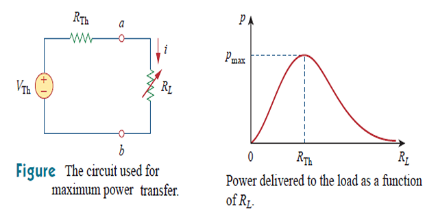
With \(R_{L}\) connected across the Thévenin equivalent, the current and the power delivered are
Both limits give zero power — at \(R_L = 0\) the voltage across the load vanishes, and as \(R_L \to \infty\) the current vanishes — so a maximum must exist in between. Differentiating with respect to \(R_{L}\) by the quotient rule:
Cancelling one factor of \(\left(R_{Th}+R_{L}\right)\) from numerator and denominator:
Setting the derivative to zero requires the numerator to vanish, giving the celebrated result
The second derivative is negative there, confirming a maximum. Substituting back gives the power delivered under the matched condition:
Maximum power transfer is emphatically not the same as maximum efficiency, and confusing the two leads to bad engineering. At the match, the load and the source resistance carry the same current and have the same resistance, so they dissipate equal power. The efficiency is therefore
Half of everything the source produces is wasted internally. This is entirely acceptable in a communication receiver, where the signal is measured in microwatts and getting the most of it matters far more than the energy cost. It would be catastrophic in a power system: no utility would deliberately dissipate half its generation in the transmission network. Power engineering therefore designs for \(R_{Th} \ll R_{L}\) and efficiencies above 95 %, accepting that the load receives far less than the theoretical maximum available.
Match for power when the source is fixed and the signal is scarce; mismatch deliberately when the energy is expensive.
Problem. For the network of Example 4.5, find the load resistance that absorbs maximum power, and the value of that power. Compare with the 4 \(\Omega\) load already considered, and with a 12 \(\Omega\) load.
Solution. From Example 4.5, \(V_{Th} = 28\) V and \(R_{Th} = 4~\Omega\). Maximum power is therefore delivered when
Verification the long way. With \(R_L = 4~\Omega\) we found \(i_L = 3.5\) A in Example 4.5, so
Comparison. With a 12 \(\Omega\) load instead,
Tripling the load resistance away from the match costs only 25 % of the deliverable power — a vivid illustration of how flat the peak is. Note too that the 12 \(\Omega\) load is the more efficient arrangement, taking 75 % of the total rather than 50 %, even though it receives less power in absolute terms.
Practical Engineering Applications
Every real source is a Thévenin equivalent. A battery, a laboratory power supply, a thermocouple, a strain-gauge bridge — each presents an open-circuit voltage and an internal resistance, and neither can be measured directly without the other. The standard experimental procedure is to measure the terminal voltage under two different known loads and solve for both parameters.
The internal resistance determines how much the terminal voltage droops as the load draws current — the regulation of the source. A car battery must have an internal resistance of a few milliohms to deliver hundreds of amperes to a starter motor without collapsing; a 9 V alkaline cell has an internal resistance of a few ohms and is quite unable to do so.
Problem. A battery measures 12.00 V on open circuit. When it supplies 3 A to a load, its terminal voltage falls to 11.40 V. Find its internal resistance, and the maximum power it could ever deliver.
Solution. The open-circuit reading is \(V_{Th}\) directly, since a voltmeter draws negligible current. The drop under load is the internal \(iR\):
The maximum deliverable power, at a matched 0.2 \(\Omega\) load, is
This would require a load current of \(12/(0.4) = 30\) A and would waste another 180 W inside the battery — which is why the matched condition is a theoretical limit here, not an operating point. The short-circuit current, incidentally, would be \(12/0.2 = 60\) A, and the internal dissipation of 720 W is exactly why shorting a battery is dangerous.
The Wheatstone bridge measures an unknown resistance by comparison rather than by reading a meter, and it is far more precise than an ohmmeter because it relies on detecting zero rather than on the accuracy of a deflection. Four resistors form two voltage dividers across a common supply, with a sensitive galvanometer between their midpoints.
The bridge is balanced when the two midpoints are at the same potential, so the galvanometer reads zero. Since both dividers see the same supply, this requires the two divider ratios to be equal:
The supply voltage cancels out entirely, so its stability is irrelevant — a considerable practical advantage. Only the ratio of the known resistors and the null detection matter, and both can be made extremely accurate.
When the bridge is not balanced, Thévenin's theorem is the natural tool: replace the bridge as seen by the galvanometer with its Thévenin equivalent and compute the deflection current directly. That calculation is the basis of every strain gauge, load cell and resistance thermometer in industrial use, where the bridge is deliberately operated slightly off balance and the imbalance is the measurement.
Summary and Key Formulas
Linearity comprises homogeneity (scaling) and additivity. All the theorems of this chapter require it, and none apply to non-linear circuits.
Power is not linear, so superposition may never be applied to power.
Superposition: sum the responses to each independent source acting alone. Voltage sources are shorted, current sources opened, and dependent sources are never deactivated.
Source transformation exchanges \(v_s\) in series with \(R\) for \(i_s = v_s/R\) in parallel with the same \(R\). Ideal sources cannot be transformed.
Thévenin: any linear two-terminal network equals \(V_{Th}\) in series with \(R_{Th}\), where \(V_{Th} = v_{oc}\).
Norton: the same network equals \(I_N = i_{sc}\) in parallel with \(R_N = R_{Th}\). The two equivalents differ by one source transformation.
\(R_{Th}\) may be found by deactivation (independent sources only), by \(v_{oc}/i_{sc}\), or by the test-source method when dependent sources are present.
Maximum power is transferred when \(R_L = R_{Th}\), giving \(p_{\max} = V_{Th}^2/4R_{Th}\) at an efficiency of exactly 50 %.
A practical source is modelled by its open-circuit voltage and internal resistance; a Wheatstone bridge balances when \(R_1/R_2 = R_3/R_x\).
| Result | Formula | Conditions |
|---|---|---|
| Homogeneity | \(x \to kx \Rightarrow y \to ky\) | linear circuits only |
| Superposition | \(y = y_1 + y_2 + \cdots\) | voltages and currents, never power |
| Source transformation | \(v_s = i_s R\) | finite non-zero \(R\) |
| Thévenin voltage | \(V_{Th} = v_{oc}\) | terminals open |
| Norton current | \(I_N = i_{sc}\) | terminals shorted |
| Equivalence relation | \(V_{Th} = I_N R_N\), \(R_{Th} = R_N\) | always |
| \(R_{Th}\) by deactivation | series/parallel reduction | independent sources only |
| \(R_{Th}\) by ratio | \(R_{Th} = \dfrac{v_{oc}}{i_{sc}}\) | always valid |
| \(R_{Th}\) by test source | \(R_{Th} = \dfrac{v_{test}}{i_{test}}\) | independent sources deactivated |
| Load power | \(p = \dfrac{V_{Th}^2 R_L}{(R_{Th}+R_L)^2}\) | any \(R_L\) |
| Matched condition | \(R_L = R_{Th}\) | maximum power, not efficiency |
| Maximum power | \(p_{\max} = \dfrac{V_{Th}^2}{4R_{Th}}\) | at the match |
| Efficiency | \(\eta = \dfrac{R_L}{R_{Th}+R_L}\) | 50 % at the match |
| Terminal voltage | \(v = V_{Th} - iR_{Th}\) | practical source |
| Bridge balance | \(R_x = \dfrac{R_2R_3}{R_1}\) | galvanometer reads zero |
Common Mistakes
Superposing powers. The single most common error in this chapter. Sum the voltages or currents first, then compute power once from the total.
Deactivating a dependent source during superposition or when finding \(R_{Th}\). Only independent sources are ever deactivated. A dependent source is part of the network's character, not an input to it.
Reversing the deactivation rules. Voltage source → short, current source → open. Setting a source's value to zero is what determines which; a zero-voltage element is a wire and a zero-current element is a break.
Getting the current-source direction wrong in a source transformation. The arrow points towards what was the positive terminal.
Trying to transform an ideal source. With no series or parallel resistance the transformation is undefined.
Leaving the load connected while finding \(V_{Th}\) or \(R_{Th}\). The equivalent describes the network without the load; the load is reconnected only at the end.
Assuming \(R_{Th}\) must be smaller than the resistances present. With dependent sources it can be much larger, or negative.
Confusing maximum power transfer with maximum efficiency. The match gives the most power at exactly 50 % efficiency — a deliberate design choice for signals, a serious mistake for power.
Applying maximum power transfer when the load is fixed and the source is adjustable. The theorem assumes \(R_{Th}\) fixed and \(R_L\) variable. If it is the other way round, the power rises monotonically as \(R_{Th}\) falls, and there is no interior optimum.
Applying any of these theorems to a non-linear circuit. A diode or a saturating core invalidates every result in this chapter.
Chapter Review
Work these before opening the answers. Where a circuit is fully solved, use the power balance as a check.
P4.1 In a linear circuit a 15 V source produces an output current of 0.6 A. What output does a 25 V source produce, all else unchanged?
Show answer
By homogeneity the response scales with the source:\[i = 0.6 \times \frac{25}{15} = 1.000~\mathrm{A}\]P4.2 An 18 V source in series with 6 \(\Omega\) feeds a node; a 3 \(\Omega\) resistor connects the node to ground and a 2 A source injects into it. Find the node voltage by superposition.
Show answer
18 V alone (open the 2 A source) — a voltage divider:2 A alone (short the 18 V source) — the resistors are in parallel:\[v' = 18 \times \frac{3}{6+3} = 6~\mathrm{V}\]\[v'' = 2 \times (6 \parallel 3) = 2 \times 2 = 4~\mathrm{V}\]Check by nodal: \(\frac{18-v}{6}+2=\frac{v}{3}\) gives \(18-v+12=2v\), so \(v=10\) V \(\checkmark\).\[v = 6 + 4 = 10~\mathrm{V}\]P4.3 Convert a 20 V source in series with 5 \(\Omega\) into its Norton form, and a 6 A source in parallel with 3 \(\Omega\) into its Thévenin form.
Show answer
\[i_s = \frac{20}{5} = 4~\mathrm{A} \ \text{in parallel with}\ 5~\Omega\]\[v_s = (6)(3) = 18~\mathrm{V} \ \text{in series with}\ 3~\Omega\]P4.4 A 36 V source in series with 12 \(\Omega\) feeds terminals \(a\)–\(b\), with a 6 \(\Omega\) resistor across those terminals. Find the Thévenin equivalent.
Show answer
\[V_{Th} = 36 \times \frac{6}{12+6} = 12~\mathrm{V}, \qquad R_{Th} = 12 \parallel 6 = \frac{72}{18} = 4~\Omega\]P4.5 Find the Norton equivalent of the network in P4.4.
Show answer
Directly: shorting \(a\)–\(b\) shorts the 6 \(\Omega\), so \(i_{sc} = 36/12 = 3\) A \(\checkmark\).\[I_N = \frac{V_{Th}}{R_{Th}} = \frac{12}{4} = 3~\mathrm{A}, \qquad R_N = 4~\Omega\]P4.6 For the network of P4.4, find the load resistance for maximum power transfer, the maximum power, and the efficiency at that point.
Show answer
\[R_L = R_{Th} = 4~\Omega, \qquad p_{\max} = \frac{12^{2}}{4(4)} = \frac{144}{16} = 9~\mathrm{W}, \qquad \eta = 50\%\]P4.7 A network consists of a 6 \(\Omega\) resistor between terminals \(a\) and \(b\), together with a dependent current source of value \(0.5v_{ab}\) flowing from \(a\) to \(b\). Find \(R_{Th}\).
Show answer
Apply a 1 V test source, so \(v_{ab} = 1\) V. The test current is the sum of both branch currents:\[i_{test} = \frac{1}{6} + 0.5(1) = 0.1667 + 0.5 = 0.6667~\mathrm{A}\]Here the dependent source aids the test current, so \(R_{Th}\) comes out well below the 6 \(\Omega\) present — the opposite of Example 4.7.\[R_{Th} = \frac{1}{0.6667} = 1.500~\Omega\]P4.8 A Wheatstone bridge balances with \(R_1 = 10~\mathrm{k}\Omega\), \(R_2 = 20~\mathrm{k}\Omega\) and \(R_3 = 15~\mathrm{k}\Omega\). Find \(R_x\).
Show answer
Note that the supply voltage plays no part — the balance condition is a ratio.\[R_x = \frac{R_2R_3}{R_1} = \frac{(20)(15)}{10} = 30~\mathrm{k}\Omega\]P4.9 A power supply reads 24.0 V open circuit and 23.2 V when delivering 4 A. Find its internal resistance and its short-circuit current.
Show answer
\[R_{Th} = \frac{24.0-23.2}{4} = \frac{0.8}{4} = 0.2000~\Omega\]In practice the supply's current limit would intervene long before this.\[i_{sc} = \frac{24.0}{0.2} = 120.0~\mathrm{A}\]P4.10 A source with \(R_{Th} = 50~\Omega\) drives a 200 \(\Omega\) load. What fraction of the maximum available power does the load receive, and what is the efficiency?
Show answer
\[\frac{p}{p_{\max}} = \frac{4R_{Th}R_L}{(R_{Th}+R_L)^{2}} = \frac{4(50)(200)}{(250)^{2}} = \frac{40\,000}{62\,500} = 0.6400\]The load receives 64 % of the available power at 80 % efficiency — a better engineering compromise than the match for most purposes.\[\eta = \frac{200}{250} = 80.00\%\]
MCQ 1. Superposition may be applied to find:
(a) power (b) voltage and current (c) energy (d) all of theseShow answer
(b) voltage and current. Power and energy are quadratic in the sources and cannot be superposed.MCQ 2. To deactivate an independent current source, replace it by:
(a) a short circuit (b) an open circuit (c) a 1 \(\Omega\) resistor (d) a voltage sourceShow answer
(b) an open circuit. Zero current means no path — the reverse rule applies to voltage sources.MCQ 3. During superposition, dependent sources are:
(a) shorted (b) opened (c) left active (d) halvedShow answer
(c) left active in every sub-circuit, with the controlling variable recomputed each time.MCQ 4. The Thévenin voltage of a network equals its:
(a) short-circuit current (b) open-circuit voltage (c) source voltage (d) load voltageShow answer
(b) open-circuit voltage, measured with the load removed.MCQ 5. A network has \(v_{oc} = 20\) V and \(i_{sc} = 4\) A. Its Thévenin resistance is:
(a) 80 \(\Omega\) (b) 5 \(\Omega\) (c) 0.2 \(\Omega\) (d) 24 \(\Omega\)Show answer
(b) 5 \(\Omega\). \(R_{Th} = v_{oc}/i_{sc} = 20/4\).MCQ 6. A 24 V source in series with 8 \(\Omega\) transforms to a current source of:
(a) 3 A in parallel with 8 \(\Omega\) (b) 3 A in series with 8 \(\Omega\) (c) 192 A in parallel with 8 \(\Omega\) (d) 8 A in parallel with 3 \(\Omega\)Show answer
(a) 3 A in parallel with 8 \(\Omega\). The resistance is unchanged and moves from series to parallel.MCQ 7. Maximum power is transferred to the load when:
(a) \(R_L = 0\) (b) \(R_L = R_{Th}\) (c) \(R_L \to \infty\) (d) \(R_L = 2R_{Th}\)Show answer
(b) \(R_L = R_{Th}\). Both extremes give zero power.MCQ 8. The efficiency of power transfer at the matched condition is:
(a) 100 % (b) 75 % (c) 50 % (d) 25 %Show answer
(c) 50 %. Equal resistances carrying the same current dissipate equal power.MCQ 9. A network with \(V_{Th} = 20\) V and \(R_{Th} = 5~\Omega\) can deliver a maximum power of:
(a) 80 W (b) 40 W (c) 20 W (d) 400 WShow answer
(c) 20 W. \(p_{\max} = V_{Th}^2/4R_{Th} = 400/20\). Option (a) is the total power drawn from the source at the match.MCQ 10. The Wheatstone bridge is precise mainly because:
(a) it uses a very accurate supply (b) it detects a null rather than a deflection (c) it uses four resistors (d) it draws no currentShow answer
(b) it detects a null. The balance condition is a ratio in which the supply voltage cancels entirely.
Superposition follows from linearity, yet power cannot be superposed even in a perfectly linear circuit. Reconcile these two statements.
Explain physically why a dependent source must not be deactivated during superposition, using the analogy of a resistor.
The Thévenin equivalent reproduces the original network exactly at its terminals. In what respect does it not reproduce the original — and why does that not matter for load calculations?
Why is \(R_{Th} = v_{oc}/i_{sc}\) the only method available when measuring a real piece of equipment on the bench?
A student argues that since maximum power transfer occurs at \(R_L = R_{Th}\), transmission lines should be designed so that their resistance equals the load resistance. Explain what is wrong with this reasoning.
Under what circumstances can a Thévenin resistance be negative, and what does a negative value tell you about what the network can do?
Part 1 has so far dealt only with resistors, and every equation in it has been algebraic. That is about to change. Chapter 5 introduces the operational amplifier — still a resistive analysis, but one in which a dependent source with enormous gain produces behaviour that seems at first to defy intuition. Chapter 6 then introduces the capacitor and the inductor, elements whose \(v\)–\(i\) relations involve derivatives and integrals rather than simple proportionality.
From that point on, circuits have memory: their present behaviour depends on their past, the equations become differential, and the response takes time to settle. The theorems of this chapter survive the transition intact — Thévenin and Norton reappear in Chapter 10 with impedances in place of resistances — but the arithmetic becomes complex, in both senses of the word.