- State the definition of the Laplace transform and explain its region of convergence.
- Derive the transforms of the step, exponential, impulse and sinusoid from the definition.
- Apply the properties — linearity, scaling, time and frequency shift, differentiation, integration — to build transforms without integrating.
- Use the initial and final value theorems to extract limiting behaviour directly from \(F(s)\).
- Invert \(F(s)\) by partial fractions for simple, repeated and complex poles.
- Handle complex poles by completing the square.
- Define the convolution integral and use the theorem \(\mathcal{L}\left[f_{1}*f_{2}\right] = F_{1}F_{2}\).
- Evaluate a convolution graphically by folding, displacing, multiplying and integrating.
- Solve integro-differential equations with initial conditions built in.
Introduction
The phasor of Chapter 9 was a remarkable device: it converted differential equations into algebraic ones and made the whole of Part 1's machinery available for AC analysis. But it had three limitations, and each was severe.
It described only the steady state, discarding the transient entirely. It handled only sinusoidal excitation, so a step, a pulse or an arbitrary waveform was outside its reach. And it could not accommodate initial conditions, which had to be treated separately by the natural-plus-forced decomposition of Chapters 7 and 8.
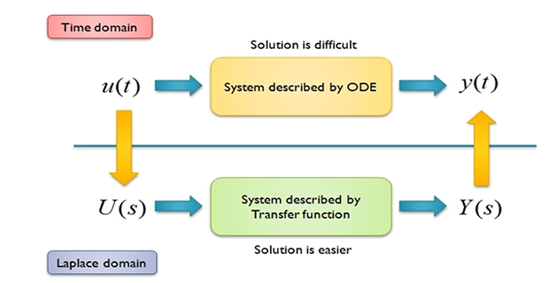
The Laplace transform removes all three restrictions at a stroke. It generalises \(j\omega\) to the complex variable \(s = \sigma + j\omega\), where the real part \(\sigma\) represents exponential growth or decay and the imaginary part \(\omega\) represents oscillation as before. A sinusoid is the special case \(\sigma = 0\), so the whole of Part 2 falls out as a special case on setting \(s = j\omega\).
The gain is more than convenience. Differential equations become algebraic equations in \(s\), and — the crucial point — the initial conditions appear automatically in the transform of the derivative. There is no separate step for them, no natural response to add to a forced response. One transformation, one algebraic solve, one inversion.
This chapter develops the transform itself. Chapter 16 applies it to circuits, where it will turn out that \(R\), \(L\) and \(C\) have impedances in the \(s\)-domain just as they had in the phasor domain — and initial conditions appear as extra sources.
Definition and Convergence
The Laplace transform is an integral transformation of \(f(t)\) from the time domain into the complex frequency domain:
Several features of this definition deserve comment.
The units of \(s\). The argument \(st\) of the exponential must be dimensionless, so \(s\) has units of inverse seconds — frequency. Hence the name complex frequency.
The lower limit is \(0^{-}\), not 0. This includes the origin itself, so any discontinuity or impulse occurring at \(t = 0\) is captured. It also means the initial conditions used are those just before switching, which is exactly what the continuity conditions of Chapter 6 provide.
The result is a definite integral, so \(t\) is integrated out and \(F(s)\) depends on \(s\) alone. Time has been eliminated, exactly as the phasor eliminated it.
This is the one-sided or unilateral transform, which ignores \(f(t)\) for \(t < 0\) — equivalently, it transforms \(f(t)u(t)\). The two-sided transform runs from \(-\infty\), but for circuit analysis, where something is switched on at a definite instant, the one-sided version is what we need.
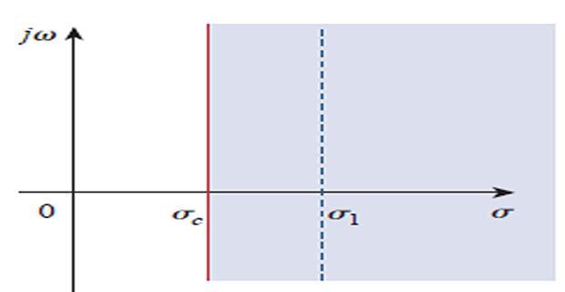
Not every function has a Laplace transform. The integral must converge to a finite value, which requires
Since \(e^{-\sigma t}\) decays faster for larger \(\sigma\), if the integral converges for some \(\sigma = \sigma_{c}\) it converges for every larger value too. Hence
The half-plane to the right of \(\sigma_{c}\) is the region of convergence, and \(F(s)\) is undefined outside it.
In practice the region of convergence rarely needs explicit attention in circuit work, because the functions encountered are all well behaved and the transform pairs are looked up rather than integrated. It matters in principle, however, because it is what makes the transform of a growing exponential possible at all — something no phasor could represent.
The inverse transform is formally a contour integral in the complex plane:
This is almost never evaluated directly. Sections 15.6 to 15.8 give the practical method: break \(F(s)\) into standard pieces by partial fractions and look each one up.
Transforms of Basic Functions
Four transforms, derived directly from the definition, generate almost everything else.
The unit step. With \(f(t) = u(t) = 1\) for \(t > 0\):
The exponential.
Note that the step is the special case \(a = 0\).
The impulse. Here the sifting property of Section 7.5 does all the work:
The impulse transforms to unity — the simplest possible \(F(s)\), and the reason the impulse response characterises a whole system. This is where the \(0^{-}\) lower limit earns its keep: with a lower limit of \(0^{+}\) the impulse would fall outside the range of integration and the transform would be zero.
The sinusoid. Writing the sine in exponential form via Euler's identity:
Each term is an exponential transform:
and the cosine follows the same way as \(s/\left(s^{2}+\omega^{2}\right)\).
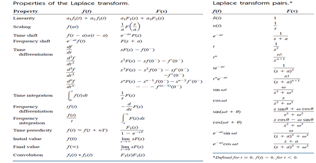
| \(f(t)\), \(t \ge 0\) | \(F(s)\) | \(f(t)\), \(t \ge 0\) | \(F(s)\) |
|---|---|---|---|
| \(\delta(t)\) | \(1\) | \(e^{-at}\sin\omega t\) | \(\dfrac{\omega}{\left(s+a\right)^{2}+\omega^{2}}\) |
| \(u(t)\) | \(\dfrac{1}{s}\) | \(e^{-at}\cos\omega t\) | \(\dfrac{s+a}{\left(s+a\right)^{2}+\omega^{2}}\) |
| \(t\) | \(\dfrac{1}{s^{2}}\) | \(t\,e^{-at}\) | \(\dfrac{1}{\left(s+a\right)^{2}}\) |
| \(t^{n}\) | \(\dfrac{n!}{s^{n+1}}\) | \(\dfrac{t^{n-1}e^{-at}}{\left(n-1\right)!}\) | \(\dfrac{1}{\left(s+a\right)^{n}}\) |
| \(e^{-at}\) | \(\dfrac{1}{s+a}\) | \(u(t-a)\) | \(\dfrac{e^{-as}}{s}\) |
| \(\sin\omega t\) | \(\dfrac{\omega}{s^{2}+\omega^{2}}\) | \(t\sin\omega t\) | \(\dfrac{2\omega s}{\left(s^{2}+\omega^{2}\right)^{2}}\) |
| \(\cos\omega t\) | \(\dfrac{s}{s^{2}+\omega^{2}}\) | \(t\cos\omega t\) | \(\dfrac{s^{2}-\omega^{2}}{\left(s^{2}+\omega^{2}\right)^{2}}\) |
Properties of the Transform
The properties are what make the transform practical: they let almost any transform be built from the table without ever performing an integration.
| Property | Statement |
|---|---|
| Linearity | \(\mathcal{L}\left[a_{1}f_{1}+a_{2}f_{2}\right] = a_{1}F_{1}(s)+a_{2}F_{2}(s)\) |
| Scaling | \(\mathcal{L}\left[f(at)\right] = \dfrac{1}{a}F\left(\dfrac{s}{a}\right)\) |
| Time shift | \(\mathcal{L}\left[f(t-a)u(t-a)\right] = e^{-as}F(s)\) |
| Frequency shift | \(\mathcal{L}\left[e^{-at}f(t)u(t)\right] = F(s+a)\) |
| Time differentiation | \(\mathcal{L}\left[\dfrac{df}{dt}\right] = sF(s)-f(0^{-})\) |
| Time integration | \(\mathcal{L}\left[\displaystyle\int_{0}^{t}f(\tau)d\tau\right] = \dfrac{1}{s}F(s)\) |
| Frequency differentiation | \(\mathcal{L}\left[t\,f(t)\right] = -\dfrac{dF(s)}{ds}\) |
| Periodic function | \(F(s) = \dfrac{F_{1}(s)}{1-e^{-Ts}}\), \(F_{1}\) from the first period |
The differentiation property is the one that matters most, and its general form for the \(n\)th derivative is
Notice what has happened. Differentiation becomes multiplication by \(s\), exactly as it became multiplication by \(j\omega\) for phasors. But now the initial conditions appear as extra terms in the same equation. They are not a separate problem to be solved afterwards; they are built in from the start. This is the single greatest advantage of the Laplace method over everything that preceded it.
Note also that \(f(0^{-})\) is used, matching the lower limit of the definition — and matching the pre-switching values that the continuity conditions of Chapter 6 supply.
The time-shift property deserves a warning. To use \(\mathcal{L}\left[f(t-a)u(t-a)\right] = e^{-as}F(s)\), the function must be expressed entirely in terms of \((t-a)\). A term such as \(t\,u(t-1)\) is not in that form and must first be rewritten as \((t-1)u(t-1) + u(t-1)\), as Example 15.3 demonstrates.
Problem. Find the Laplace transform of \(f(t) = \delta(t) + 2u(t) - 3e^{-2t}u(t)\).
Solution. Linearity allows term-by-term transformation:
Combining over a common denominator:
Either form is acceptable; the separated form is more useful for inversion, the combined form for identifying poles. Here the poles are at \(s = 0\) and \(s = -2\), corresponding to the constant and the decaying exponential.
Problem. Find the transform of \(g(t) = 10\left[u(t-2)-u(t-3)\right]\) — a pulse of height 10 lasting from \(t=2\) to \(t=3\).
Solution. Each step is already in shifted form, so the time-shift property applies directly with \(F(s) = 1/s\) for the unit step:
This is the pattern for any pulse: a delay of \(a\) seconds contributes a factor \(e^{-as}\), and nothing else. The exponentials in \(s\) are the signature of time delays, and recognising them on sight is worth cultivating.
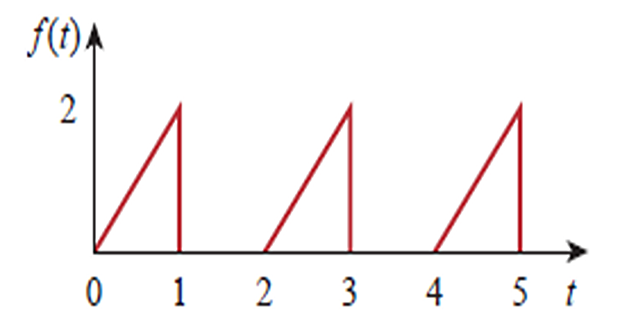
Problem. Find the transform of a periodic function of period \(T = 2\) whose first period is \(f_{1}(t) = 2t\left[u(t)-u(t-1)\right]\) — a ramp rising to 2 over one second, then zero for one second.
Step 1 — transform the first period. Expand and rewrite the shifted term so that the time-shift property can be used:
The second term is not in the required form, so add and subtract 1 inside:
Now every term is either unshifted or expressed purely in \((t-1)\). Using \(\mathcal{L}\left[t\right] = 1/s^{2}\) and the shift property:
Step 2 — apply the periodicity property.
Why the periodicity formula works. A periodic function is its first period plus the same shifted by \(T\), plus again by \(2T\), and so on. Transforming gives \(F_{1}\left(1+e^{-Ts}+e^{-2Ts}+\cdots\right)\), and the geometric series sums to \(1/\left(1-e^{-Ts}\right)\). An infinite sum in the time domain collapses to a single division in the \(s\)-domain.
Initial and Final Value Theorems
Two theorems extract the behaviour of \(f(t)\) at the extremes of time directly from \(F(s)\), without inverting it at all.
The correspondence is intuitive once noticed: large \(s\) corresponds to small \(t\) and vice versa, since \(s\) has units of inverse time.
These theorems are excellent checks. Having inverted an \(F(s)\) by partial fractions, evaluate the two limits and confirm they match the initial and final values of the answer. Any algebraic slip in the residues will usually show up immediately.
A caution about the final value theorem. It is valid only if \(f(\infty)\) actually exists — that is, if all poles of \(sF(s)\) lie in the left half-plane. Applying it to a function that oscillates forever or grows without bound gives a meaningless number. For \(F(s) = \omega/\left(s^{2}+\omega^{2}\right)\), for instance, the theorem returns 0, yet \(\sin\omega t\) has no final value at all. The initial value theorem carries no such restriction.
Problem. Find the initial and final values of the function whose transform is
Initial value. Multiply by \(s\) and let \(s\to\infty\). Dividing numerator and denominator by the highest power makes the limit clear:
Final value. Multiply by \(s\) and let \(s\to 0\):
Both limits are zero, so \(h(t)\) starts at zero and returns to zero — a transient that rises and decays. The final value theorem is legitimate here because the poles are at \(s = -3\) and \(s = -4\pm j3\), all in the left half-plane.
Example 15.7 inverts this same \(H(s)\) completely and confirms both limits.
Inverse Transform: Simple Poles
Inversion in practice means partial fraction expansion: break \(F(s)\) into a sum of terms each of which appears in the table, then invert term by term using linearity.
For distinct poles \(p_{i}\), and provided the degree of the numerator is less than that of the denominator,
The constants \(k_{i}\) are the residues, and each is found by the cover-up rule: multiply through by the corresponding factor and evaluate at that pole, which annihilates every other term.
Each term then inverts to an exponential:
Each pole contributes one exponential, whose decay rate is the pole's location. A pole far to the left decays fast; a pole near the origin decays slowly; a pole at the origin gives a constant. A pole in the right half-plane would give a growing exponential — which is why stability is a question about pole locations, as Chapter 16 will make explicit.
If the numerator degree is not less than the denominator's, divide out first: long division leaves a proper fraction plus a polynomial in \(s\), whose terms invert to \(\delta(t)\) and its derivatives.
Problem. Find the inverse transform of \(F(s) = \dfrac{s^{2}+12}{s\left(s+2\right)\left(s+3\right)}\).
Solution. Three distinct poles at \(s = 0, -2, -3\), so
Applying the cover-up rule to each in turn:
Check with the theorems. Final value: \(\lim_{s\to0}sF(s) = 12/6 = 2\), and indeed \(f(\infty) = 2\) since both exponentials vanish \(\checkmark\). Initial value: \(\lim_{s\to\infty}sF(s) = 1\), and \(f(0) = 2-8+7 = 1\) \(\checkmark\). Both agree, so the residues are right.
Repeated Poles
A pole repeated \(n\) times requires \(n\) terms, one for each power up to \(n\):
where \(F_{1}(s)\) collects the remaining, non-repeated part. The highest-order residue comes from the cover-up rule as before, but the others require successive differentiation:
The differentiation is needed because simply covering up would leave the lower-order terms still present at \(s = -p\); differentiating first removes them.
The inversion uses the pair
so a repeated pole produces terms like \(te^{-at}\) and \(t^{2}e^{-at}\). These are exactly the forms met in the critically damped case of Chapter 8, where the repeated root of the characteristic equation forced an extra factor of \(t\). The Laplace method now explains why that factor appears: a repeated pole demands it.
Problem. Find the inverse transform of \(V(s) = \dfrac{10s^{2}+4}{s\left(s+1\right)\left(s+2\right)^{2}}\).
Solution. Two simple poles and one double pole, so four terms:
The three cover-up residues:
The remaining residue requires differentiation. Note that \(s(s+1) = s^{2}+s\):
At \(s = -2\): \(s^{2}+s = 2\), \(20s = -40\), \(10s^{2}+4 = 44\) and \(2s+1 = -3\), so
Check. Final value: \(\lim_{s\to0}sV(s) = 4/4 = 1\), matching \(v(\infty) = 1\) \(\checkmark\). Initial value: \(\lim_{s\to\infty}sV(s) = 0\), and \(v(0) = 1-14+13+0 = 0\) \(\checkmark\). Note the \(te^{-2t}\) term produced by the double pole.
Complex Poles
A pair of complex conjugate poles is simple if not repeated, and could in principle be handled by the cover-up rule. In practice the complex algebra is cumbersome, and a better method is completing the square.
Write the quadratic factor and its numerator as
and complete the square in the denominator:
so that \(\alpha = a/2\) and \(\beta = \sqrt{b-\alpha^{2}}\). Then split the numerator to match the two standard forms:
Both terms are now in the table, giving
A complex pole pair produces a damped sinusoid, with \(\alpha\) — the real part — setting the decay and \(\beta\) — the imaginary part — setting the oscillation frequency. Comparing with Chapter 8, \(\alpha\) is the damping factor and \(\beta\) the damped natural frequency \(\omega_{d}\). The underdamped response is precisely what a complex pole pair looks like.
The cosine and sine terms can be merged into a single cosine with a phase angle, using the identity of Section 8.4:
Problem. Find the inverse transform of \(H(s) = \dfrac{20}{\left(s+3\right)\left(s^{2}+8s+25\right)}\) — the function whose limiting values were found in Example 15.4.
Step 1 — set up the expansion. One real pole and one complex pair:
The complex poles themselves are at
Step 2 — find \(B\) and \(C\) by substituting convenient values. Cover-up will not work for the quadratic, so equate the two sides at any two values of \(s\). Taking \(s = 0\):
and taking \(s = 1\):
Step 3 — complete the square. Here \(\alpha = 4\) and \(\beta^{2} = 25-16 = 9\), so \(\beta = 3\):
Splitting the second term and arranging the sine numerator to be exactly \(\beta = 3\):
Step 4 — combine into a single cosine.
Check against Example 15.4. At \(t = 0\): \(2 - 2 - 0 = 0\) \(\checkmark\), matching the initial value theorem. As \(t\to\infty\) both exponentials vanish, giving 0 \(\checkmark\). The response is a decaying exponential plus a damped oscillation at 3 rad/s — the signature of the complex pair at \(-4\pm j3\).
The Convolution Integral
If a system's response to an impulse is \(h(t)\), its response to an arbitrary input \(x(t)\) is given by the convolution integral. For a causal system driven by a signal starting at \(t=0\):
The limits deserve explanation. The lower limit is 0 because \(x(t) = 0\) for \(t < 0\). The upper limit is \(t\) because the system is causal: \(h(t) = 0\) for negative argument, so \(h(t-\lambda) = 0\) whenever \(\lambda > t\). A system cannot respond to an input it has not yet received, and that physical fact is what truncates the integral.
Properties. Convolution behaves much like multiplication:
| Property | Statement |
|---|---|
| Commutative | \(x*h = h*x\) |
| Distributive | \(f*\left(x+y\right) = f*x + f*y\) |
| Associative | \(f*\left(x*y\right) = \left(f*x\right)*y\) |
| Impulse is the identity | \(f*\delta(t) = f(t)\) |
| Shifted impulse delays | \(f*\delta\left(t-t_{0}\right) = f\left(t-t_{0}\right)\) |
| Impulse derivative | \(f*\delta'(t) = f'(t)\) |
| Step integrates | \(f*u(t) = \displaystyle\int_{-\infty}^{t}f(\lambda)d\lambda\) |
That the impulse is the identity element explains why \(h(t)\) is called the impulse response: convolving any input with an impulse returns the input unchanged, so a system whose impulse response is an impulse passes everything through untouched.
The connection to the Laplace transform is the reason convolution appears in this chapter at all:
Convolution in the time domain is multiplication in the \(s\)-domain. A difficult integral becomes a trivial product, which is normally the easier route by a wide margin: transform both functions, multiply, and invert.
Two situations where the time-domain route is still preferable:
When the product \(F_{1}(s)F_{2}(s)\) is complicated enough that inverting it is harder than doing the integral.
When \(f_{1}\) or \(f_{2}\) is available only as measured data, with no closed form and hence no explicit transform.
The second case is the common one in practice, and it is why numerical convolution remains a standard tool in signal processing.

Graphical Convolution
The convolution of two signals is best understood graphically, and for piecewise-constant signals the graphical method is often the fastest route to an answer. There are four steps.
Folding. Take the mirror image of \(h(\lambda)\) about the vertical axis to obtain \(h(-\lambda)\).
Displacement. Shift \(h(-\lambda)\) to the right by \(t\) to obtain \(h(t-\lambda)\).
Multiplication. Form the product \(h(t-\lambda)\,x(\lambda)\).
Integration. For that value of \(t\), find the area under the product for \(0 < \lambda < t\). That area is \(y(t)\).
Repeating for every \(t\) traces out the whole response. The mnemonic is fold, shift, multiply, integrate.
In practice the work is organised by identifying the ranges of \(t\) over which the overlap pattern is qualitatively the same, then computing one integral per range. The number of ranges is determined by the breakpoints of the two signals.

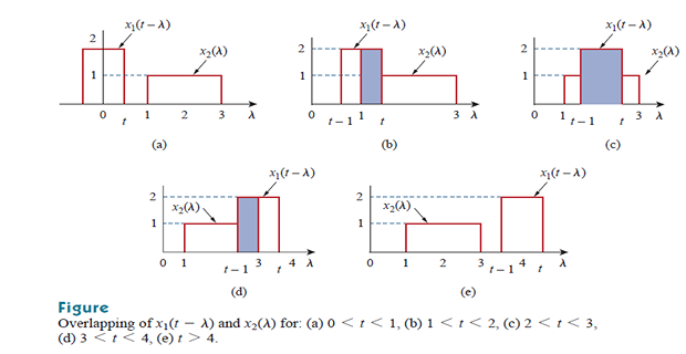
Problem. Find \(y(t) = x_{1}(t)*x_{2}(t)\), where \(x_{1}\) is a pulse of height 2 and width 1 starting at \(t=0\), and \(x_{2}\) is a pulse of height 1 extending from \(t=1\) to \(t=3\).
Solution. Fold \(x_{1}\) and shift it by \(t\). Since the folded pulse has width 1 and the stationary pulse occupies \(1 \le \lambda \le 3\), four ranges arise.
Range 1, \(0 < t < 1\). The shifted pulse has not yet reached \(\lambda = 1\), so there is no overlap:
Range 2, \(1 < t < 2\). Partial overlap, growing. The overlap runs from \(\lambda = 1\) to \(\lambda = t\):
Range 3, \(2 < t < 3\). Complete overlap — the whole of the moving pulse lies inside the stationary one:
Range 4, \(3 < t < 4\). Overlap shrinking as the pulse leaves. It runs from \(\lambda = t-1\) to \(\lambda = 3\):
Range 5, \(t > 4\). No overlap remains, so \(y(t) = 0\). Collecting:
Three checks. The result is continuous at every breakpoint — at \(t=2\) both expressions give 2, and at \(t=3\) both give 2. Its total duration is \(4-1 = 3\), the sum of the two individual durations (1 and 2), which is always true of a convolution. And its area is \(4\), equal to the product of the two individual areas \(\left(2\times1\right)\times\left(1\times2\right)\) — also always true.
Convolving two rectangles gives a trapezoid; convolving two rectangles of equal width would give a triangle. This is the general pattern, and it is worth recognising.


Problem. An RL circuit has the transfer function \(H(s) = \mathbf{I}_{o}/\mathbf{I}_{s} = 1/\left(s+1\right)\). Find its response to the pulse \(i_{s}(t) = u(t)-u(t-2)~\mathrm{A}\) using the convolution integral.
Solution. The impulse response is the inverse transform of \(H(s)\):
Treat the two step terms separately.
First term, active for all \(t > 0\). Since \(e^{-t}\) is constant with respect to \(\lambda\) it comes outside:
Second term, active only for \(t > 2\), with the integration starting at \(\lambda = 2\):
Subtracting the second from the first for \(t > 2\), and noting that for \(t < 2\) only the first contributes:
Check the continuity at \(t = 2\). From the left, \(1-e^{-2} = 0.8647\); from the right, \(\left(e^{2}-1\right)e^{-2} = 1-e^{-2} = 0.8647\) \(\checkmark\). The two expressions agree exactly, as they must for an inductor current, which cannot jump.
The physical picture is the RL step response of Chapter 7: the current rises towards 1 A while the pulse is present, reaching 86.5 % of its final value after two time constants, then decays exponentially once the source is removed.


Integro-Differential Equations
The differentiation and integration properties together turn any linear integro-differential equation with constant coefficients into an algebraic equation. The procedure has three steps:
Transform the equation term by term, using \(\mathcal{L}\left[f'\right] = sF-f(0^{-})\) and \(\mathcal{L}\left[\int f\right] = F/s\). The initial conditions enter here automatically.
Solve algebraically for the transform of the unknown.
Invert by partial fractions.
Compare this with Chapters 7 and 8, where the natural response had to be found from the characteristic equation, the forced response from the steady state, the two added, and the arbitrary constants fitted to the initial conditions afterwards. The Laplace method does all of that in one pass, and it never requires the response to be classified as over-, critically or underdamped — the partial fraction expansion sorts that out by itself, according to whether the poles turn out to be real, repeated or complex.
Problem. Solve \(\dfrac{d^{2}x}{dt^{2}}+5\dfrac{dx}{dt}+6x = 0\) subject to \(x(0) = 2\) and \(x'(0) = -1\).
Step 1 — transform. Using the derivative property for both terms:
Substituting the initial conditions:
Step 2 — solve algebraically.
Note that the denominator is exactly the characteristic polynomial of Chapter 8 — the poles are the natural frequencies \(s_{1} = -2\) and \(s_{2} = -3\).
Step 3 — invert.
Check both initial conditions.
Both are satisfied automatically — they were never fitted afterwards, because they entered the algebra at step 1. That is the whole point of the method, and it is why the Laplace transform supersedes the classical approach for every problem in the rest of this book.
Summary and Key Formulas
The Laplace transform maps \(f(t)\) into \(F(s)\) with \(s = \sigma+j\omega\), generalising the phasor's \(j\omega\) to include exponential growth and decay.
The lower limit \(0^{-}\) captures impulses and discontinuities at the origin and matches the pre-switching initial conditions.
The transform exists where the integral converges, in a right half-plane \(\mathrm{Re}(s) > \sigma_{c}\).
Differentiation becomes multiplication by \(s\), with the initial conditions appearing automatically; integration becomes division by \(s\).
A delay of \(a\) seconds contributes a factor \(e^{-as}\); a periodic function's transform is its first period divided by \(1-e^{-Ts}\).
The initial and final value theorems give limiting behaviour without inversion, the latter valid only if the final value exists.
Inversion is by partial fractions: simple poles give exponentials, repeated poles give \(t^{n}e^{-at}\) terms, and complex pairs give damped sinusoids.
Complex poles are best handled by completing the square, with \(\alpha\) giving the decay and \(\beta\) the oscillation frequency.
Convolution in time equals multiplication in \(s\); graphically it is fold, shift, multiply, integrate.
Integro-differential equations become algebraic ones, solved in a single pass with no separate natural and forced parts.
| Result | Formula | Notes |
|---|---|---|
| Definition | \(F(s) = \displaystyle\int_{0^{-}}^{\infty}f(t)e^{-st}dt\) | one-sided |
| Convergence | \(\mathrm{Re}(s) > \sigma_{c}\) | right half-plane |
| Step | \(\mathcal{L}\left[u(t)\right] = 1/s\) | |
| Exponential | \(\mathcal{L}\left[e^{-at}\right] = 1/(s+a)\) | |
| Impulse | \(\mathcal{L}\left[\delta(t)\right] = 1\) | needs \(0^{-}\) limit |
| Sine and cosine | \(\dfrac{\omega}{s^{2}+\omega^{2}}\), \(\dfrac{s}{s^{2}+\omega^{2}}\) | |
| Time shift | \(\mathcal{L}\left[f(t-a)u(t-a)\right] = e^{-as}F(s)\) | express in \((t-a)\) first |
| Frequency shift | \(\mathcal{L}\left[e^{-at}f(t)\right] = F(s+a)\) | |
| First derivative | \(sF(s)-f(0^{-})\) | initial condition built in |
| \(n\)th derivative | \(s^{n}F - s^{n-1}f(0^{-}) - \cdots - f^{(n-1)}(0^{-})\) | |
| Integration | \(\mathcal{L}\left[\displaystyle\int_{0}^{t}f\,d\tau\right] = F(s)/s\) | |
| Periodic function | \(F(s) = \dfrac{F_{1}(s)}{1-e^{-Ts}}\) | geometric series |
| Initial value | \(f(0^{+}) = \lim_{s\to\infty}sF(s)\) | always valid |
| Final value | \(f(\infty) = \lim_{s\to0}sF(s)\) | only if it exists |
| Simple pole residue | \(k_{i} = \left.\left(s+p_{i}\right)F(s)\right|_{s=-p_{i}}\) | cover-up rule |
| Repeated pole residue | \(k_{n-m} = \dfrac{1}{m!}\left.\dfrac{d^{m}}{ds^{m}}\left[\left(s+p\right)^{n}F\right]\right|_{s=-p}\) | |
| Repeated pole inverse | \(\mathcal{L}^{-1}\left[\dfrac{1}{\left(s+a\right)^{n}}\right] = \dfrac{t^{n-1}e^{-at}}{\left(n-1\right)!}\) | gives \(te^{-at}\) etc. |
| Complex poles | \(\left(s+\alpha\right)^{2}+\beta^{2}\) | complete the square |
| Complex pole inverse | \(\left(A_{1}\cos\beta t+B_{1}\sin\beta t\right)e^{-\alpha t}\) | damped sinusoid |
| Convolution | \(y(t) = \displaystyle\int_{0}^{t}x(\lambda)h(t-\lambda)d\lambda\) | causal, \(t \ge 0\) |
| Convolution theorem | \(\mathcal{L}\left[f_{1}*f_{2}\right] = F_{1}(s)F_{2}(s)\) | time \(\to\) product |
Common Mistakes
Applying the time-shift property to a function not expressed in \((t-a)\). \(t\,u(t-1)\) must first be rewritten as \((t-1)u(t-1)+u(t-1)\), as in Example 15.3.
Omitting the initial-condition terms in the derivative property. \(\mathcal{L}\left[f'\right]\) is \(sF(s)-f(0^{-})\), not simply \(sF(s)\). Dropping them silently assumes zero initial conditions.
Using the final value theorem when no final value exists. For an oscillating or growing function the limit returns a number that means nothing. Check the pole locations first.
Forgetting the differentiation step for repeated poles. Only the highest-order residue comes from a plain cover-up; the rest need derivatives.
Failing to make the sine numerator equal \(\beta\). The table entry is \(\beta/\left[\left(s+\alpha\right)^{2}+\beta^{2}\right]\), so a numerator of 2 with \(\beta = 3\) must be written as \(\tfrac{2}{3}\times3\).
Applying partial fractions to an improper fraction. If the numerator degree is not less than the denominator's, divide out first.
Using \(f(0^{+})\) where the property calls for \(f(0^{-})\). They differ whenever an impulse acts at the origin, which is exactly when it matters.
Getting the convolution limits wrong. They are 0 to \(t\) for a causal system driven from rest — not \(-\infty\) to \(\infty\), and not 0 to \(\infty\).
Forgetting to fold before shifting. The integrand is \(h(t-\lambda)\), which is \(h\) reversed and then displaced.
Convolving when multiplying transforms would be easier. Unless the data are numerical or the product is intractable, transform first.
Chapter Review
Work these before opening the answers. Where an inverse transform is found, check it with the initial and final value theorems.
P15.1 Find the Laplace transform of \(f(t) = 4\delta(t)-3u(t)+5e^{-4t}u(t)\).
Show answer
\[F(s) = 4 - \frac{3}{s} + \frac{5}{s+4}\]P15.2 Find the transform of a rectangular pulse of height 5 lasting from \(t = 1\) to \(t = 4\).
Show answer
\[f(t) = 5\left[u(t-1)-u(t-4)\right] \;\Longrightarrow\; F(s) = \frac{5}{s}\left(e^{-s}-e^{-4s}\right)\]P15.3 Find the initial and final values for \(F(s) = \dfrac{6\left(s+2\right)}{s\left(s+1\right)\left(s+4\right)}\).
Show answer
\[f(0^{+}) = \lim_{s\to\infty}\frac{6s\left(s+2\right)}{s\left(s+1\right)\left(s+4\right)} = 0\]Both poles of \(sF(s)\) are in the left half-plane, so the final value is legitimate.\[f(\infty) = \lim_{s\to0}\frac{6\left(s+2\right)}{\left(s+1\right)\left(s+4\right)} = \frac{12}{4} = 3\]P15.4 Invert \(F(s) = \dfrac{6\left(s+2\right)}{s\left(s+1\right)\left(s+4\right)}\) and verify against P15.3.
Show answer
\[A = \frac{6\left(2\right)}{\left(1\right)\left(4\right)} = 3, \qquad B = \frac{6\left(1\right)}{\left(-1\right)\left(3\right)} = -2, \qquad C = \frac{6\left(-2\right)}{\left(-4\right)\left(-3\right)} = -1\]Check: \(f(0) = 3-2-1 = 0\) \(\checkmark\) and \(f(\infty) = 3\) \(\checkmark\)\[f(t) = \left(3 - 2e^{-t} - e^{-4t}\right)u(t)\]P15.5 Invert \(F(s) = \dfrac{8}{s\left(s+2\right)^{2}}\).
Show answer
\[F(s) = \frac{A}{s}+\frac{C}{\left(s+2\right)^{2}}+\frac{D}{s+2}\]\[A = \frac{8}{4} = 2, \qquad C = \left.\frac{8}{s}\right|_{s=-2} = -4, \qquad D = \left.\frac{d}{ds}\left(\frac{8}{s}\right)\right|_{s=-2} = \left.\frac{-8}{s^{2}}\right|_{s=-2} = -2\]Check: \(f(0) = 2-0-2 = 0\) \(\checkmark\), \(f(\infty) = 2\) \(\checkmark\)\[f(t) = \left(2 - 4te^{-2t} - 2e^{-2t}\right)u(t)\]P15.6 Invert \(F(s) = \dfrac{10}{s^{2}+6s+25}\) by completing the square.
Show answer
\[s^{2}+6s+25 = \left(s+3\right)^{2}+16 \;\Longrightarrow\; \alpha = 3, \; \beta = 4\]\[F(s) = \frac{10}{\left(s+3\right)^{2}+16} = \frac{10}{4}\cdot\frac{4}{\left(s+3\right)^{2}+16}\]\[f(t) = 2.5\,e^{-3t}\sin 4t\;u(t)\]P15.7 Solve \(\dfrac{dx}{dt}+3x = 6u(t)\) with \(x(0) = 1\).
Show answer
\[sX-1+3X = \frac{6}{s} \;\Longrightarrow\; X(s) = \frac{6}{s\left(s+3\right)}+\frac{1}{s+3} = \frac{s+6}{s\left(s+3\right)}\]\[A = \frac{6}{3} = 2, \qquad B = \frac{-3+6}{-3} = -1\]Check: \(x(0) = 1\) \(\checkmark\) and \(x(\infty) = 2 = 6/3\) \(\checkmark\) — the universal first-order formula of Chapter 7 in disguise.\[x(t) = \left(2 - e^{-3t}\right)u(t)\]P15.8 Use the convolution theorem to find \(\mathcal{L}^{-1}\left[\dfrac{1}{s\left(s+1\right)}\right]\) two ways.
Show answer
By convolution: the factors invert to \(u(t)\) and \(e^{-t}\), soBy partial fractions: \(\dfrac{1}{s}-\dfrac{1}{s+1}\), giving the same result \(\checkmark\) The partial-fraction route is shorter, which is typical.\[f(t) = \int_{0}^{t}\left(1\right)e^{-(t-\lambda)}d\lambda = e^{-t}\left(e^{t}-1\right) = 1-e^{-t}\]P15.9 Two rectangular pulses, each of unit height and width 2, are convolved. Sketch the result and state its peak value, duration and area.
Show answer
Equal-width rectangles convolve to a triangle. Peak value 2 (the overlap length at full coincidence), duration \(2+2 = 4\), and area \(\left(1\times2\right)\times\left(1\times2\right) = 4\).
Check: a triangle of base 4 and height 2 has area \(\tfrac{1}{2}\left(4\right)\left(2\right) = 4\) \(\checkmark\)P15.10 A system has \(H(s) = \dfrac{2}{s+4}\). Find its impulse response and its step response.
Show answer
Impulse response: \(h(t) = 2e^{-4t}u(t)\).
Step response: multiply by \(1/s\) and invert:Note that the step response is the integral of the impulse response, since dividing by \(s\) is integration.\[Y(s) = \frac{2}{s\left(s+4\right)} = \frac{0.5}{s}-\frac{0.5}{s+4} \;\Longrightarrow\; y(t) = 0.5\left(1-e^{-4t}\right)u(t)\]
MCQ 1. The Laplace transform of \(\delta(t)\) is:
(a) \(1/s\) (b) 1 (c) \(s\) (d) 0Show answer
(b) 1, by the sifting property. Option (a) is the step.MCQ 2. The lower limit of the defining integral is \(0^{-}\) in order to:
(a) simplify the algebra (b) capture impulses at the origin (c) ensure convergence (d) match the upper limitShow answer
(b). With a limit of \(0^{+}\), \(\mathcal{L}\left[\delta(t)\right]\) would be 0.MCQ 3. \(\mathcal{L}\left[df/dt\right]\) equals:
(a) \(sF(s)\) (b) \(sF(s)-f(0^{-})\) (c) \(F(s)/s\) (d) \(F(s)+f(0^{-})\)Show answer
(b). The initial condition appears automatically — the method's chief advantage.MCQ 4. A time delay of \(a\) seconds corresponds in the \(s\)-domain to:
(a) \(F(s+a)\) (b) \(F(s-a)\) (c) \(e^{-as}F(s)\) (d) \(F(s)/a\)Show answer
(c). Option (a) is the frequency shift, produced by multiplying by \(e^{-at}\) in time.MCQ 5. A double pole at \(s = -a\) produces a time-domain term of the form:
(a) \(e^{-at}\) (b) \(te^{-at}\) (c) \(e^{-2at}\) (d) \(\cos at\)Show answer
(b) \(te^{-at}\), the critically damped form of Chapter 8.MCQ 6. A complex conjugate pole pair at \(-\alpha \pm j\beta\) gives:
(a) two exponentials (b) a damped sinusoid (c) a constant (d) a rampShow answer
(b), oscillating at \(\beta\) inside an envelope \(e^{-\alpha t}\) — the underdamped response.MCQ 7. The final value theorem may be applied only when:
(a) \(F(s)\) is proper (b) the final value exists (c) all poles are real (d) alwaysShow answer
(b). All poles of \(sF(s)\) must lie in the left half-plane; otherwise the limit is meaningless.MCQ 8. Convolution in the time domain corresponds in the \(s\)-domain to:
(a) addition (b) multiplication (c) convolution (d) divisionShow answer
(b) multiplication. This is why transforming is usually easier than convolving.MCQ 9. The four steps of graphical convolution are:
(a) shift, fold, add, differentiate (b) fold, shift, multiply, integrate (c) multiply, fold, shift, add (d) integrate, fold, shift, multiplyShow answer
(b). The folding comes first because the integrand contains \(h(t-\lambda)\).MCQ 10. Convolving two rectangular pulses of equal width gives:
(a) a rectangle (b) a triangle (c) a trapezoid (d) an exponentialShow answer
(b) a triangle. Unequal widths give a trapezoid, as in Example 15.8.
The phasor and the Laplace transform both convert differential equations into algebraic ones. Identify precisely what the Laplace transform can do that the phasor cannot, and say what is given up in exchange.
Why must the lower limit of the defining integral be \(0^{-}\) rather than \(0^{+}\)? Give a concrete function for which the choice changes the answer.
Every pole of \(F(s)\) contributes a term to \(f(t)\). Explain what a pole in the right half-plane would mean physically, and why circuit designers care about pole locations.
Chapter 8 required the response to be classified as over-, critically or underdamped before it could be written down. The Laplace method requires no such classification. Explain how the classification nonetheless emerges.
The convolution integral has limits 0 to \(t\) rather than \(-\infty\) to \(\infty\). Identify the two physical assumptions responsible, and describe a system for which one of them fails.
Convolving two signals produces an output lasting as long as the sum of their durations, with area equal to the product of their areas. Justify both statements without algebra.
The transform is now in hand as a piece of mathematics. Chapter 16 turns it on circuits, and the result is the most powerful analysis method in the book.
Each element acquires an \(s\)-domain impedance — \(R\) for a resistor, \(sL\) for an inductor, \(1/sC\) for a capacitor — exactly parallel to the phasor impedances of Chapter 9, with \(s\) in place of \(j\omega\). Initial conditions appear as additional sources in the transformed circuit, so a charged capacitor becomes a capacitor plus a voltage source and an energised inductor becomes an inductor plus a source.
Everything then proceeds as in Chapter 10: nodal analysis, mesh analysis, Thévenin, superposition — all unchanged, all now handling transients and initial conditions in a single pass. The transfer function \(\mathbf{H}(s)\) returns, its poles determining stability and transient behaviour, and setting \(s = j\omega\) recovers the frequency response of Chapter 14.