- Define the transfer function \(\mathbf{H}(\omega)\) and obtain its magnitude and phase.
- Work in decibels, distinguishing the power and voltage forms.
- Construct Bode plots using straight-line asymptotes for gains, poles, zeros and quadratic factors.
- Determine the resonant frequency of series and parallel RLC circuits.
- Compute the quality factor, bandwidth and half-power frequencies, and relate them.
- Explain selectivity and the trade-off between high \(Q\) and wide bandwidth.
- Recognise and design the four passive filter types.
- Design first-order active filters using op amps.
- Apply magnitude and frequency scaling to convert a normalised prototype into a practical design.
Introduction
Every circuit in Part 2 was driven at a single fixed frequency. Impedances were computed once, the circuit was solved, and that was the end of it. This chapter asks a different question: what happens as the frequency is varied?
The answer reshapes the subject. Since \(\mathbf{Z}_{L} = j\omega L\) grows without limit as frequency rises while \(\mathbf{Z}_{C} = 1/j\omega C\) shrinks towards zero, any circuit containing both has one particular frequency at which the two cancel exactly. At that resonant frequency the circuit becomes purely resistive and its response reaches a sharp extremum.
The parameter \(\omega_{0} = 1/\sqrt{LC}\) that appeared in Chapter 8 as the undamped natural frequency of a transient turns out to be precisely this resonant frequency — the same number, seen from the frequency domain instead of the time domain. The damping ratio reappears too, inverted, as the quality factor that determines how sharp the resonance is.
From resonance follow filters — circuits designed to pass certain frequencies and reject others — and with them the whole of communications engineering. And to display how a circuit behaves across many decades of frequency at once, we need the Bode plot and the logarithmic decibel scale it is drawn on.
The Transfer Function
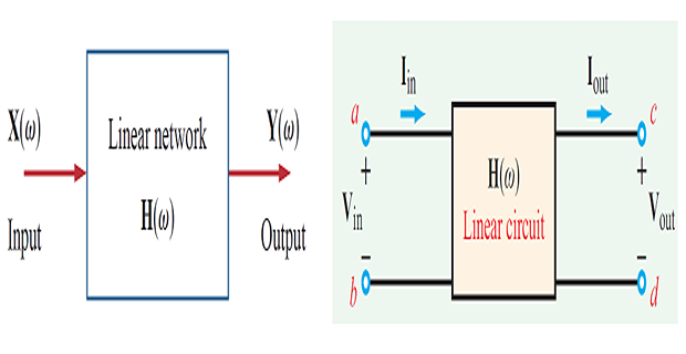
The transfer function \(\mathbf{H}(\omega)\) is the ratio of a circuit's output phasor to its input phasor, as a function of frequency.
Since input and output may each be a voltage or a current, there are four kinds:
| Transfer function | Definition | Units |
|---|---|---|
| Voltage gain | \(\mathbf{V}_{o}/\mathbf{V}_{i}\) | dimensionless |
| Current gain | \(\mathbf{I}_{o}/\mathbf{I}_{i}\) | dimensionless |
| Transfer impedance | \(\mathbf{V}_{o}/\mathbf{I}_{i}\) | ohms |
| Transfer admittance | \(\mathbf{I}_{o}/\mathbf{V}_{i}\) | siemens |
Being a ratio of complex quantities, \(\mathbf{H}\) is itself complex and is written
where \(H\) is the magnitude response and \(\phi\) the phase response. Plotting both against frequency gives the frequency response, and that pair of plots is the complete description of what a linear circuit does to any sinusoid.
Written as a ratio of polynomials in \(j\omega\),
the roots of \(\mathbf{N} = 0\) are the zeros and the roots of \(\mathbf{D} = 0\) the poles. A pole makes the response large; a zero makes it small. Locating them is the quickest way to see what a circuit will do.
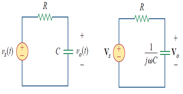
Problem. A series RC circuit has the output taken across the capacitor, with \(R = 10~\mathrm{k}\Omega\) and \(C = 0.1~\mu\mathrm{F}\). Obtain \(\mathbf{H}(\omega) = \mathbf{V}_{o}/\mathbf{V}_{s}\), its magnitude and phase, and evaluate them at several frequencies.
Solution. By voltage division with impedances:
Defining \(\omega_{0} = 1/RC\) puts this in standard form:
| \(\omega/\omega_{0}\) | \(H\) | \(H\) in dB | \(\phi\) |
|---|---|---|---|
| 0 | 1.000 | 0 | 0° |
| 0.1 | 0.9950 | −0.043 | −5.71° |
| 1 | 0.7071 | −3.010 | −45° |
| 2 | 0.4472 | −6.990 | −63.43° |
| 10 | 0.09950 | −20.04 | −84.29° |
| \(\infty\) | 0 | −∞ | −90° |
The circuit passes low frequencies unchanged and progressively attenuates high ones — a low-pass filter. The row at \(\omega = \omega_{0}\) is the important one: the magnitude has fallen to \(1/\sqrt{2}\), the gain is exactly \(-3\) dB, and the phase is exactly \(-45^{\circ}\). That triple coincidence defines the cutoff or half-power frequency, and it recurs throughout the chapter.
The Decibel Scale
Frequency responses span enormous ranges — a filter may pass one frequency at unity gain and reject another by a factor of a million. A logarithmic scale is essential, and the one universally used comes from telephone engineering.
The bel measures a power ratio as its logarithm:
The bel proved too large for convenience, so the decibel — one tenth of a bel — is used instead:
The voltage form. If the two powers are developed in equal resistances, then \(P = V^{2}/R\) and
The factor is 10 for power ratios and 20 for voltage or current ratios. Confusing them is the commonest error with decibels, and it produces an answer exactly double or half the correct one. Strictly the voltage form requires equal resistances; in practice it is applied to any voltage ratio, and the convention is universal.
| Ratio | Power (dB) | Voltage (dB) | Note |
|---|---|---|---|
| 1 | 0 | 0 | no change |
| \(\sqrt{2}\) | 1.505 | 3.010 | the "3 dB point" |
| 2 | 3.010 | 6.021 | doubling |
| 10 | 10 | 20 | one decade |
| 100 | 20 | 40 | |
| 1000 | 30 | 60 | |
| \(1/\sqrt{2} = 0.7071\) | −1.505 | −3.010 | half power |
The row worth memorising is \(1/\sqrt{2}\). A voltage ratio of 0.7071 is \(-3\) dB, and since power goes as the square, the power has fallen to exactly one half. This is why the −3 dB point and the half-power point are the same thing, and why cutoff frequencies are quoted at \(-3\) dB.
The great convenience of decibels is that cascaded stages add instead of multiplying, since the logarithm of a product is the sum of the logarithms. This is what makes Bode plots possible.
Problem. (a) Express a power gain of 100 and a voltage gain of 100 in decibels. (b) A signal chain has an amplifier of \(+20\) dB, a second of \(+15\) dB, and a cable loss of 6 dB. Find the overall gain in decibels and as a voltage ratio. (c) What voltage ratio corresponds to \(-3\) dB?
(a)
The same numerical ratio gives different decibel values depending on which quantity it describes — hence the need to state which.
(b) Decibels add along a chain:
Multiplying the individual ratios would give \(10 \times 5.623 \times 0.5012 = 28.18\) — the same, but with far more arithmetic.
(c)
and the corresponding power ratio is \(\left(0.7071\right)^{2} = 0.5\) — half power, as expected.
Bode Plots
Bode plots are semilogarithmic plots of magnitude in decibels and phase in degrees against frequency on a logarithmic axis. Their power comes from a single observation: on a logarithmic magnitude scale, the factors of a transfer function add rather than multiply, so each may be plotted separately and the results summed graphically.
To exploit this, the transfer function is first written in standard form, in which every factor is arranged as \(\left(1+j\omega/\text{something}\right)\):
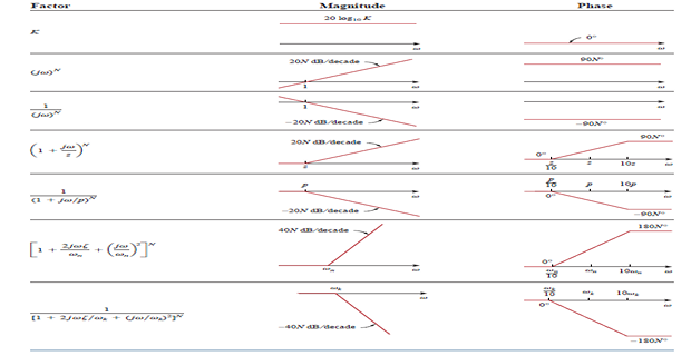
Only four kinds of factor can appear, and each has a simple asymptotic plot:
a constant gain \(K\);
a pole or zero at the origin, \(\left(j\omega\right)^{\pm1}\);
a simple pole or zero, \(\left(1+j\omega/p\right)^{-1}\) or \(\left(1+j\omega/z\right)\);
a quadratic pole or zero.
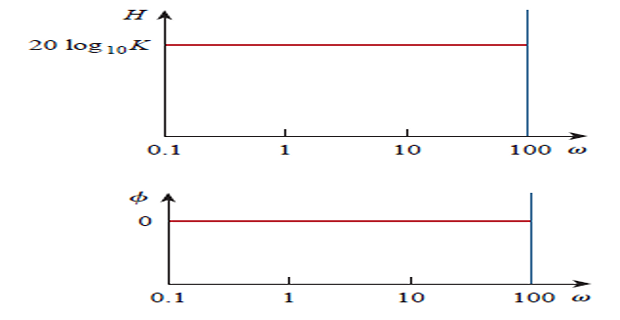
Constant gain \(K\). Magnitude \(20\log_{10}K\) and phase \(0^{\circ}\), both flat with frequency. A negative \(K\) leaves the magnitude unchanged but shifts the phase by \(\pm180^{\circ}\).
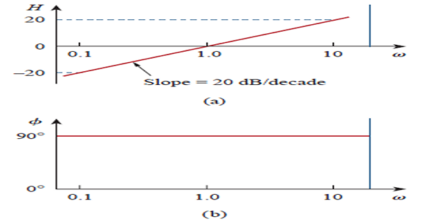
Zero at the origin, \(\left(j\omega\right)\). Magnitude \(20\log_{10}\omega\) — a straight line of slope +20 dB/decade passing through 0 dB at \(\omega = 1\) — and constant phase \(+90^{\circ}\). A pole at the origin gives \(-20\) dB/decade and \(-90^{\circ}\). For \(\left(j\omega\right)^{N}\) the figures become \(20N\) dB/decade and \(90N\) degrees.
A decade is an interval between two frequencies in the ratio 10 — say 10 Hz to 100 Hz. "20 dB per decade" means the magnitude changes by 20 dB for every tenfold change in frequency.
Simple zero \(\left(1+j\omega/z_{1}\right)\). The magnitude is \(20\log_{10}\left|1+j\omega/z_{1}\right|\), which has two asymptotes:
A flat line at 0 dB for low frequencies and a line of slope \(+20\) dB/decade for high ones. The two meet at \(\omega = z_{1}\), called the corner or break frequency.
The approximation's error is largest exactly at the corner, where the true value is
so the straight-line construction is 3 dB low there — the same 3 dB that defines the cutoff frequency, and not a coincidence.
The phase runs from \(0^{\circ}\) to \(90^{\circ}\), passing through \(45^{\circ}\) at the corner. The straight-line approximation takes it as 0° below \(z_{1}/10\), 90° above \(10z_{1}\), and a straight ramp between — a slope of 45° per decade.
Simple pole \(1/\left(1+j\omega/p_{1}\right)\). Identical but inverted: slope \(-20\) dB/decade above the corner, phase falling to \(-90^{\circ}\), and the true curve 3 dB below the asymptote at the corner.
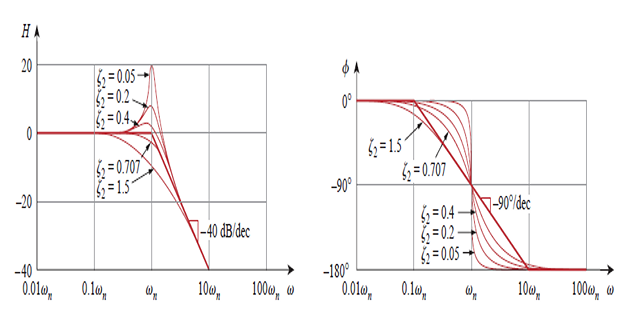
Quadratic pole. For \(1/\left[1+j2\zeta\omega/\omega_{n}+\left(j\omega/\omega_{n}\right)^{2}\right]\) the asymptotes are 0 dB below \(\omega_{n}\) and \(-40\) dB/decade above it, with the phase running from 0° through \(-90^{\circ}\) at \(\omega_{n}\) to \(-180^{\circ}\).
Here the straight-line approximation can be seriously wrong. The true curve depends on the damping ratio \(\zeta\) of Chapter 8, and for small \(\zeta\) there is a pronounced peak near \(\omega_{n}\) that the asymptotes miss entirely. The asymptotic plot is exactly the same as for a double pole \(\left(1+j\omega/\omega_{n}\right)^{-2}\), which is the case \(\zeta = 1\); any other \(\zeta\) requires a correction near the corner.
| Factor | Magnitude slope | Phase | Corner |
|---|---|---|---|
| \(K\) | flat at \(20\log_{10}K\) | 0° (or 180° if \(K<0\)) | — |
| \(\left(j\omega\right)\) | \(+20\) dB/dec throughout | \(+90^{\circ}\) | 0 dB at \(\omega=1\) |
| \(\left(j\omega\right)^{-1}\) | \(-20\) dB/dec throughout | \(-90^{\circ}\) | 0 dB at \(\omega=1\) |
| \(1+j\omega/z\) | 0, then \(+20\) dB/dec | 0° to \(+90^{\circ}\) | \(\omega = z\) |
| \(\left(1+j\omega/p\right)^{-1}\) | 0, then \(-20\) dB/dec | 0° to \(-90^{\circ}\) | \(\omega = p\) |
| quadratic zero | 0, then \(+40\) dB/dec | 0° to \(+180^{\circ}\) | \(\omega = \omega_{k}\) |
| quadratic pole | 0, then \(-40\) dB/dec | 0° to \(-180^{\circ}\) | \(\omega = \omega_{n}\) |
The procedure: put \(\mathbf{H}\) in standard form, identify every factor, mark all corner frequencies on the log axis, start from the low-frequency asymptote, and change the slope by the appropriate amount at each corner as you move right.
Problem. Construct the Bode plots for
Step 1 — standard form. Factor 2 from the first bracket and 10 from the second, so each becomes \(1+j\omega/\ldots\):
Four factors are now visible: a gain of 10, a zero at the origin, and simple poles at \(\omega = 2\) and \(\omega = 10\).
Step 2 — magnitude and phase in additive form.
Step 3 — assemble the slopes. Working left to right along the frequency axis:
| Range | Active factors | Net slope |
|---|---|---|
| \(\omega < 2\) | gain + origin zero | \(+20\) dB/dec |
| \(2 < \omega < 10\) | pole at 2 now active | \(0\) dB/dec (flat) |
| \(\omega > 10\) | both poles active | \(-20\) dB/dec |
Rising, flat, then falling — this is a band-pass response.
Step 4 — check some exact values.
| \(\omega\) (rad/s) | \(H\) | dB | \(\phi\) |
|---|---|---|---|
| 0.5 | 4.845 | 13.71 | 73.10° |
| 2 | 13.87 | 22.84 | 33.69° |
| 4.472 | 16.67 | 24.44 | 0° |
| 10 | 13.87 | 22.84 | −33.69° |
| 100 | 1.990 | 5.976 | −83.14° |
The peak occurs at exactly \(\omega = \sqrt{2\times10} = \sqrt{20} = 4.472\) rad/s — the geometric mean of the two corner frequencies — where the two arctangents cancel and the phase is precisely zero. The peak magnitude is \(50/3 = 16.67\), or 24.44 dB.
That the response is real at its peak is not an accident: it is the resonance condition of the next section, appearing here in a circuit that is not obviously an RLC one. Note also the symmetry of the table about \(\omega = 4.472\) on a logarithmic axis — 2 and 10 give the same magnitude, as do 0.5 and 40.
Series Resonance
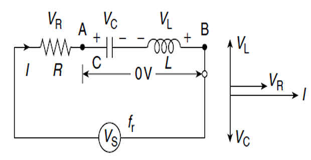
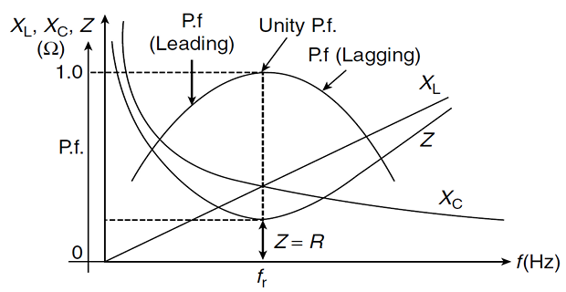
Resonance is the condition in which a circuit's impedance is purely real — the inductive and capacitive reactances cancel exactly, leaving voltage and current in phase.
For a series RLC circuit,
Setting the imaginary part to zero:
This is the same \(\omega_{0}\) as in Chapter 8, where it was the undamped natural frequency of the transient. The circuit's tendency to oscillate at \(1/\sqrt{LC}\) when disturbed, and its tendency to respond most strongly to excitation at \(1/\sqrt{LC}\), are the same fact viewed from two domains.
At resonance:
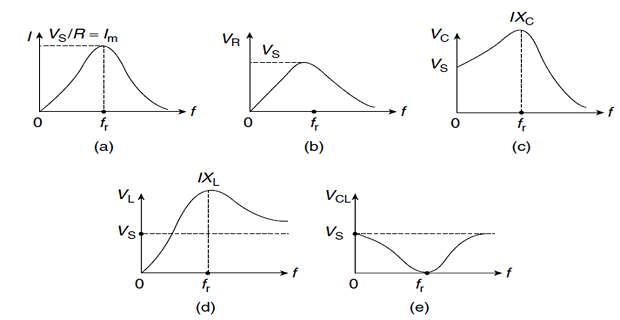
\(\mathbf{Z} = R\) — the impedance is minimum and purely resistive, so the current is maximum.
The \(LC\) pair behaves as a short circuit, and the entire source voltage appears across \(R\).
Voltage and current are in phase, so the power factor is unity.
The average power dissipated is at its maximum, \(P(\omega_{0}) = \tfrac{1}{2}V_{m}^{2}/R\).
A striking consequence. Although the reactances cancel, they are individually far from zero. The voltage across each is
where \(Q\) is the quality factor defined in the next section. The voltage across the inductor and across the capacitor can be many times the source voltage — they are equal in magnitude and opposite in phase, so they cancel in the KVL sum while each individually is enormous. A series resonant circuit is therefore also called a voltage resonant circuit, and this voltage magnification is a real hazard: components must be rated for \(QV_{m}\), not \(V_{m}\).
Quality Factor and Bandwidth
The current magnitude in a series RLC circuit is
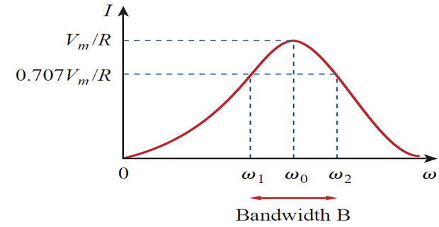
peaking at \(V_{m}/R\) when \(\omega = \omega_{0}\). At two other frequencies the dissipated power falls to half its maximum, and these are the half-power frequencies \(\omega_{1}\) and \(\omega_{2}\). Half the power means the current has fallen by \(1/\sqrt{2}\), so
Solving this quadratic gives
Multiplying the two roots reveals a neat relationship:
The resonant frequency is the geometric mean of the half-power frequencies — not the arithmetic mean, because the response is not symmetrical about \(\omega_{0}\) on a linear axis. It is symmetrical on a logarithmic axis, which is one more reason Bode plots use one.
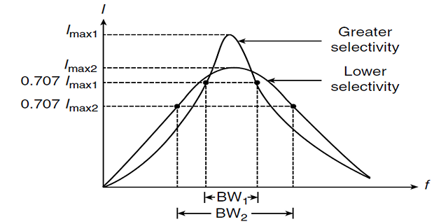
The bandwidth is the width of the half-power band:
The quality factor measures the sharpness of a resonance. Its fundamental definition is energetic:
Equivalently, it is the ratio of reactive power to real power, which for a series circuit gives
Substituting \(\omega_{0} = 1/\sqrt{LC}\) into the bandwidth expression connects the two:
High \(Q\) means narrow bandwidth. The quality factor is the ratio of the resonant frequency to the bandwidth, so a circuit with \(Q = 100\) at 1 MHz has a bandwidth of only 10 kHz.
Selectivity is the ability of a circuit to respond to one frequency band while rejecting others. A narrow band demands high \(Q\); a wide band demands low \(Q\). Since \(Q = \omega_{0}L/R\), high \(Q\) means low resistance — losses are what blunt a resonance.
A circuit with \(Q \ge 10\) is called high-Q, and for such circuits the half-power frequencies are very nearly symmetrical about \(\omega_{0}\):
A resonant circuit is completely characterised by five related parameters — \(\omega_{0}\), \(\omega_{1}\), \(\omega_{2}\), \(Q\) and \(B\) — of which any two determine the rest.
The link back to Chapter 8. For a series circuit, \(\alpha = R/2L\) and \(Q = \omega_{0}L/R\), so \(Q = \omega_{0}/2\alpha = 1/2\zeta\). The quality factor and the damping ratio are reciprocals up to a factor of two: a lightly damped circuit rings for a long time in the time domain and has a sharp peak in the frequency domain, because these are the same property.
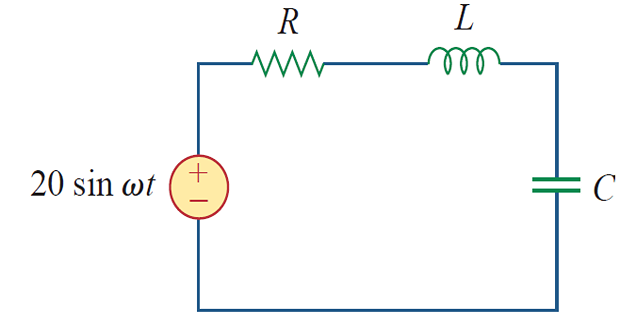
Problem. A series RLC circuit has \(R = 2~\Omega\), \(L = 1~\mathrm{mH}\) and \(C = 0.4~\mu\mathrm{F}\), driven by a source of amplitude 20 V. Find \(\omega_{0}\), \(\omega_{1}\), \(\omega_{2}\), \(Q\) and \(B\), and the current amplitude at each of the three frequencies.
Solution. The resonant frequency:
Working in krad/s throughout keeps the arithmetic manageable. With \(R/2L = 1~\mathrm{krad/s}\) and \(1/LC = 2500~\left(\mathrm{krad/s}\right)^{2}\):
Confirming by the direct formulas:
Currents. At resonance the impedance is purely \(R\):
At the half-power frequencies the current is smaller by \(\sqrt{2}\):
Since \(Q = 25 \ge 10\) this is a high-Q circuit, and indeed \(\omega_{0} \pm B/2 = 49\) and 51 krad/s, within 0.02 % of the exact values. Note the voltage magnification: \(\left|\mathbf{V}_{L}\right| = QV_{m} = 25(20) = 500~\mathrm{V}\) across the inductor, from a 20 V source.
Parallel Resonance
The parallel RLC circuit is the dual, and by the duality of Section 8.9 every result carries over with current and voltage exchanged.
Its admittance is
and setting the imaginary part to zero gives the same resonant frequency:
But the behaviour at resonance is inverted. Where the series circuit had minimum impedance and maximum current, the parallel circuit has maximum impedance and minimum current. And where the series circuit magnified voltage, the parallel circuit magnifies current: the currents circulating in \(L\) and \(C\) can be \(Q\) times the supply current, which is why it is called a current resonant or tank circuit.
| Characteristic | Series circuit | Parallel circuit |
|---|---|---|
| Resonant frequency \(\omega_{0}\) | \(\dfrac{1}{\sqrt{LC}}\) | \(\dfrac{1}{\sqrt{LC}}\) |
| Quality factor \(Q\) | \(\dfrac{\omega_{0}L}{R}\) or \(\dfrac{1}{\omega_{0}RC}\) | \(\dfrac{R}{\omega_{0}L}\) or \(\omega_{0}RC\) |
| Bandwidth \(B\) | \(\dfrac{\omega_{0}}{Q}\) | \(\dfrac{\omega_{0}}{Q}\) |
| Half-power \(\omega_{1,2}\) | \(\omega_{0}\sqrt{1+\left(\dfrac{1}{2Q}\right)^{2}} \pm \dfrac{\omega_{0}}{2Q}\) | |
| For \(Q \ge 10\) | \(\omega_{0}\pm\dfrac{B}{2}\) | \(\omega_{0}\pm\dfrac{B}{2}\) |
| At resonance | \(Z\) minimum, \(I\) maximum | \(Z\) maximum, \(I\) minimum |
| Magnifies | voltage across \(L\), \(C\) | current through \(L\), \(C\) |
Note the crucial reversal in \(Q\). For the series circuit \(Q = \omega_{0}L/R\) falls as \(R\) rises; for the parallel circuit \(Q = R/\omega_{0}L\) rises with \(R\). A large resistance sharpens a parallel resonance and blunts a series one — exactly the pattern seen with the damping factor in Chapter 8, and for the same reason.

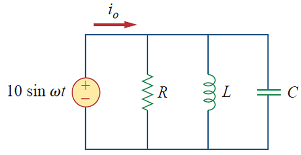
Problem. A parallel RLC circuit has \(R = 8~\mathrm{k}\Omega\), \(L = 0.2~\mathrm{mH}\) and \(C = 8~\mu\mathrm{F}\). Find \(\omega_{0}\), \(Q\), \(B\) and the half-power frequencies. If it is driven by a current source of amplitude 10 mA, find the power dissipated at each.
Solution.
Confirming with the alternative form: \(Q = \omega_{0}RC = \left(25\times10^{3}\right)\left(8000\right)\left(8\times10^{-6}\right) = 1600\) \(\checkmark\)
With \(Q = 1600\), far above 10, the approximation is excellent:
Power. At resonance the circuit is purely resistive, so all the source current flows through \(R\):
An exceptionally sharp resonance. A \(Q\) of 1600 gives a bandwidth of only 15.6 rad/s at a centre frequency of 25 000 rad/s — a fractional bandwidth of 0.06 %. Such selectivity is what a radio receiver needs to separate one station from its neighbours, and it is achievable here only because the parallel resistance is large.
Passive Filters
A filter is a circuit designed to pass signals in one band of frequencies and reject those outside it. A passive filter uses only \(R\), \(L\) and \(C\). There are four types.
| Type | Passes | Simplest realisation | Cutoff |
|---|---|---|---|
| Low-pass | \(\omega < \omega_{c}\) | series \(R\), output across \(C\) | \(\omega_{c} = 1/RC\) |
| High-pass | \(\omega > \omega_{c}\) | series \(C\), output across \(R\) | \(\omega_{c} = 1/RC\) |
| Band-pass | \(\omega_{1} < \omega < \omega_{2}\) | series RLC, output across \(R\) | \(\omega_{0} = 1/\sqrt{LC}\) |
| Band-stop | outside \(\omega_{1}\) to \(\omega_{2}\) | series RLC, output across \(LC\) | \(\omega_{0} = 1/\sqrt{LC}\) |
The transfer functions follow immediately from voltage division. For the low-pass and high-pass pair:
Their squared magnitudes sum to one at every frequency, which is why a single RC network can serve as both — take the output across the capacitor for low-pass, across the resistor for high-pass. Example 14.1 was the low-pass case.
The band-pass filter is a series resonant circuit, so everything from Sections 14.5 and 14.6 applies: its centre frequency is \(\omega_{0} = 1/\sqrt{LC}\), its bandwidth is \(B = R/L\), and its selectivity is \(Q = \omega_{0}/B\). The band-stop filter is the same circuit with the output taken from the other element, so it rejects precisely what the band-pass accepts.
Two practical limitations of passive filters. They cannot have a gain greater than one, since they contain no source of energy. And a filter's response depends on what is connected to it, so cascading two passive stages does not simply multiply their transfer functions — the second loads the first. Both problems are solved in the next section.
Problem. Design a series RLC band-pass filter with a centre frequency of 1 MHz and a bandwidth of 10 kHz, using an inductor of 100 \(\mu\mathrm{H}\). Find \(Q\), \(R\) and \(C\).
Solution. Convert to angular frequencies:
The required selectivity follows from the ratio of centre frequency to bandwidth — a ratio that may be taken in hertz or in rad/s, since the \(2\pi\) cancels:
From \(Q = \omega_{0}L/R\):
and from \(\omega_{0} = 1/\sqrt{LC}\):
A design note. The required 6.283 \(\Omega\) is small, and a real 100 \(\mu\mathrm{H}\) inductor at 1 MHz may well have that much resistance of its own. In practice the inductor's own losses often set the achievable \(Q\), and no resistor need be added at all — one simply has to accept whatever \(Q\) the coil provides. Obtaining higher \(Q\) than a coil allows requires either a quartz crystal, whose effective \(Q\) can exceed 10 000, or an active filter.
Active Filters
An active filter combines resistors and capacitors with an operational amplifier. This solves both limitations of the passive filter at once: the op amp supplies gain, and its low output impedance and high input impedance mean that stages can be cascaded without loading one another.
A third advantage matters more than either at low frequencies. Passive filters need inductors, which at audio frequencies are large, heavy, lossy and expensive. Active filters achieve the same responses with no inductors at all, which is why every audio equaliser and every anti-aliasing filter is active.
The design rests on the Chapter 5 result, extended to impedances in Section 10.11:
First-order active low-pass. Take \(\mathbf{Z}_{1} = R_{1}\) and \(\mathbf{Z}_{f} = R_{f}\parallel C_{f}\):
A low-pass response with a DC gain of \(-R_{f}/R_{1}\) — and note that the gain and the cutoff frequency are set independently, by \(R_{1}\) and \(C_{f}\) respectively. No passive filter offers that.
First-order active high-pass. Move the capacitor to the input, \(\mathbf{Z}_{1} = R_{1}+1/j\omega C_{1}\) with \(\mathbf{Z}_{f} = R_{f}\):
Band-pass by cascading. A low-pass stage followed by a high-pass stage, with the high-pass cutoff below the low-pass cutoff, passes only the band between them. Because op-amp stages do not load one another, the overall transfer function really is the product of the two — and on a Bode plot, the sum.
Higher-order responses come from cascading more stages, and the second-order Sallen–Key topology mentioned in Section 8.8 gives a quadratic pole whose damping is set by a resistor ratio rather than by a physical inductance.
Problem. Design a first-order active low-pass filter with a DC gain of 10 (inverting) and a cutoff frequency of 1592 Hz, using \(C_{f} = 1~\mathrm{nF}\).
Solution. The cutoff in angular terms:
From \(\omega_{c} = 1/R_{f}C_{f}\):
and the gain fixes the input resistor:
Check the behaviour. At DC the capacitor is an open circuit and the gain is \(-10\), or 20 dB. At \(\omega = \omega_{c}\) the magnitude is \(10/\sqrt{2} = 7.071\), which is 17 dB — exactly 3 dB down, as it must be. Above the cutoff the response falls at 20 dB/decade.
Compare this with Example 10.11, which analysed the same topology at a single frequency and obtained a gain of \(0.7071\angle135^{\circ}\). That was this filter operating exactly at its cutoff, with unity DC gain — the same circuit, now understood across all frequencies rather than at one.
Scaling
Filter designs are usually tabulated for a normalised prototype with \(R = 1~\Omega\) and \(\omega_{0} = 1~\mathrm{rad/s}\), because the algebra is then trivial. Scaling converts such a prototype into a realisable circuit at any impedance level and any frequency.
Magnitude scaling multiplies every impedance by \(K_{m}\) while leaving the frequency response unchanged. Since \(\mathbf{Z}_{R} = R\), \(\mathbf{Z}_{L} = j\omega L\) and \(\mathbf{Z}_{C} = 1/j\omega C\), this requires
Note that the capacitor scales inversely, because its impedance is inversely proportional to \(C\).
Frequency scaling shifts the response to a higher frequency by \(K_{f}\) without changing impedance levels. Each reactance must reach the same value at \(K_{f}\) times the frequency, so
Combining both gives the general result:
The resistance depends on \(K_{m}\) alone, the inductance on the ratio, and the capacitance on the product. Quality factor, damping ratio and every other dimensionless parameter are unaffected — scaling changes the numbers but never the shape of the response.
Problem. A normalised prototype has \(R = 1~\Omega\), \(L = 1~\mathrm{H}\) and \(C = 1~\mathrm{F}\), giving \(\omega_{0} = 1~\mathrm{rad/s}\). Scale it to operate at \(\omega_{0} = 10^{4}~\mathrm{rad/s}\) in a 1 \(\mathrm{k}\Omega\) system.
Solution. The two scale factors read off directly from the targets:
Applying the three rules:
Check the result.
The prototype's 1 H and 1 F are absurd as components; the scaled 0.1 H and 0.1 \(\mu\mathrm{F}\) are ordinary parts. This is the point of the technique — design once in normalised form, then scale to whatever is buildable.
Practical Engineering Applications
Tuning a radio is resonance made audible. A parallel LC circuit in the receiver's front end presents a high impedance only at its resonant frequency, so only that station's signal develops appreciable voltage. All the others — arriving at the antenna simultaneously and at comparable strength — are shunted away.
Since \(\omega_{0} = 1/\sqrt{LC}\), tuning is achieved by varying \(C\) with a fixed \(L\): historically a ganged variable capacitor, today a voltage-controlled varactor diode.
The design constraint is selectivity. Adjacent AM stations are spaced 10 kHz apart, so at 1 MHz the receiver needs \(Q \gtrsim 100\) to separate them — which is exactly the specification of Example 14.6. Too low a \(Q\) and stations interfere; too high, and the sidebands carrying the audio are themselves attenuated.
Problem. An AM receiver covers 540 kHz to 1600 kHz using a fixed inductor of 1 mH. Find the range of capacitance required.
Solution. From \(\omega_{0} = 1/\sqrt{LC}\), the capacitance needed at each end is \(C = 1/\omega_{0}^{2}L\).
At the low-frequency end:
At the high-frequency end:
So the capacitor must vary from about 9.9 pF to 86.9 pF — a ratio of
The capacitance ratio is the square of the frequency ratio, because \(C \propto 1/\omega^{2}\). This is why a variable capacitor covering the whole AM band must have such a wide range, and why FM receivers — whose band spans only 88 to 108 MHz, a ratio of 1.23 — need a capacitance ratio of just 1.5.
A single loudspeaker drive unit cannot reproduce the whole audio range: a large cone moves enough air for bass but is too heavy to follow treble, while a small one does the reverse. A crossover network splits the amplifier's output, sending low frequencies to the woofer through a low-pass filter and high frequencies to the tweeter through a high-pass one.
The simplest is a first-order pair: an inductor in series with the woofer and a capacitor in series with the tweeter, both chosen so that their cutoffs coincide at the crossover frequency, typically 2 to 3 kHz. Passive components are used despite their bulk because the network must handle the full amplifier power.
Note that both filters see the loudspeaker impedance as their load, so the design must account for it — a reminder of the loading problem that active filters avoid.
A telephone keypad encodes each key as a pair of simultaneous tones, one from a low group and one from a high group. The exchange identifies the key using a bank of band-pass filters, one per tone — a direct application of high-\(Q\) resonance. Using two tones rather than one makes accidental triggering by speech essentially impossible.
In power systems the same theory is used in reverse. A harmonic filter is a series LC branch tuned to a troublesome harmonic — typically the fifth or seventh — and connected in parallel with the supply. At its resonant frequency the branch presents nearly zero impedance, so it swallows the harmonic current before it can reach the rest of the network, while at 50 Hz it looks capacitive and conveniently contributes to power factor correction as well.
Summary and Key Formulas
The transfer function \(\mathbf{H}(\omega)\) is the output-to-input phasor ratio; its magnitude and phase plots constitute the frequency response.
Decibels use 10\(\log\) for power ratios and 20\(\log\) for voltage ratios. A voltage ratio of \(1/\sqrt{2}\) is \(-3\) dB and corresponds to half power.
Bode plots exploit the fact that logarithms add: each factor is plotted asymptotically and the results summed.
Slopes are \(\pm20\) dB/decade per simple pole or zero and \(\pm40\) for quadratics; the straight-line error at a corner is 3 dB.
Resonance occurs when the reactances cancel, at \(\omega_{0} = 1/\sqrt{LC}\) for both series and parallel circuits.
Series resonance gives minimum impedance and magnifies voltage by \(Q\); parallel resonance gives maximum impedance and magnifies current by \(Q\).
\(Q = \omega_{0}/B\), and \(\omega_{0} = \sqrt{\omega_{1}\omega_{2}}\) — the geometric mean of the half-power frequencies.
The four passive filter types are low-pass, high-pass, band-pass and band-stop; band-pass and band-stop are resonant circuits.
Active filters add gain, remove the need for inductors, and allow cascading without loading.
Scaling converts a normalised prototype to any impedance and frequency without altering the response shape.
| Result | Formula | Notes |
|---|---|---|
| Transfer function | \(\mathbf{H}(\omega) = \mathbf{Y}(\omega)/\mathbf{X}(\omega)\) | four kinds |
| Decibels, power | \(G_{\mathrm{dB}} = 10\log_{10}\left(P_{2}/P_{1}\right)\) | factor 10 |
| Decibels, voltage | \(G_{\mathrm{dB}} = 20\log_{10}\left(V_{2}/V_{1}\right)\) | factor 20 |
| Half-power point | \(1/\sqrt{2} = 0.7071 \equiv -3.010\) dB | voltage ratio |
| Simple pole/zero slope | \(\pm20\) dB/decade | above the corner |
| Quadratic slope | \(\pm40\) dB/decade | above \(\omega_{n}\) |
| Corner error | 3.010 dB | asymptote vs true |
| Resonant frequency | \(\omega_{0} = \dfrac{1}{\sqrt{LC}}\), \(f_{0} = \dfrac{1}{2\pi\sqrt{LC}}\) | series and parallel |
| Series \(Q\) | \(Q = \dfrac{\omega_{0}L}{R} = \dfrac{1}{\omega_{0}CR}\) | falls as \(R\) rises |
| Parallel \(Q\) | \(Q = \dfrac{R}{\omega_{0}L} = \omega_{0}RC\) | rises as \(R\) rises |
| Bandwidth | \(B = \omega_{2}-\omega_{1} = \dfrac{\omega_{0}}{Q}\) | series: \(B = R/L\) |
| Half-power frequencies | \(\omega_{1,2} = \mp\dfrac{R}{2L}+\sqrt{\left(\dfrac{R}{2L}\right)^{2}+\dfrac{1}{LC}}\) | series circuit |
| Geometric mean | \(\omega_{0} = \sqrt{\omega_{1}\omega_{2}}\) | always |
| High-Q approximation | \(\omega_{1,2} \simeq \omega_{0} \mp B/2\) | \(Q \ge 10\) |
| Voltage magnification | \(\left|\mathbf{V}_{L}\right| = \left|\mathbf{V}_{C}\right| = QV_{m}\) | series resonance |
| \(Q\) and damping | \(Q = 1/2\zeta\) | links to Chapter 8 |
| RC cutoff | \(\omega_{c} = 1/RC\) | low- and high-pass |
| Active low-pass | \(-\dfrac{R_{f}}{R_{1}}\cdot\dfrac{1}{1+j\omega R_{f}C_{f}}\) | gain and \(\omega_{c}\) independent |
| Magnitude scaling | \(R' = K_{m}R\), \(L' = K_{m}L\), \(C' = C/K_{m}\) | response unchanged |
| Frequency scaling | \(L' = L/K_{f}\), \(C' = C/K_{f}\) | \(R\) unchanged |
| Combined scaling | \(L' = \dfrac{K_{m}}{K_{f}}L\), \(C' = \dfrac{C}{K_{m}K_{f}}\) | ratio and product |
Common Mistakes
Using \(10\log\) for a voltage ratio. Power ratios take 10, voltage and current ratios take 20. The error is a factor of two in decibels.
Forgetting to convert to standard form before drawing a Bode plot. Every factor must read \(\left(1+j\omega/\text{corner}\right)\), so \(\left(j\omega+2\right)\) must be written \(2\left(1+j\omega/2\right)\) — and that 2 belongs in the gain term.
Confusing \(f\) and \(\omega\) in resonance formulas. \(\omega_{0} = 1/\sqrt{LC}\) is in rad/s; \(f_{0}\) is smaller by \(2\pi\). Ratios such as \(Q = \omega_{0}/B\) are safe in either unit provided both are the same.
Using the series \(Q\) formula for a parallel circuit. They are reciprocal in \(R\): series \(Q = \omega_{0}L/R\), parallel \(Q = R/\omega_{0}L\).
Taking \(\omega_{0}\) as the arithmetic mean of the half-power frequencies. It is the geometric mean. The arithmetic mean is a good approximation only for \(Q \ge 10\).
Overlooking voltage magnification at series resonance. A 20 V source across a \(Q = 25\) circuit puts 500 V across the inductor. Components must be rated accordingly.
Assuming cascaded passive filters multiply their transfer functions. The second stage loads the first. Only buffered or active stages cascade cleanly.
Applying the straight-line Bode approximation near a lightly damped quadratic pole. The true curve can peak far above the asymptotes when \(\zeta\) is small.
Scaling the capacitor the same way as the inductor. Under magnitude scaling \(L\) multiplies by \(K_{m}\) while \(C\) divides by it.
Believing a passive filter can have gain above one. It contains no energy source. Gain requires an active device.
Chapter Review
Work these before opening the answers. State clearly whether each frequency is in hertz or radians per second.
P14.1 Express as decibels: (a) a power gain of 50, (b) a voltage gain of 50, (c) a voltage gain of 0.25.
Show answer
\[\text{(a) } 10\log_{10}50 = 16.99~\mathrm{dB}, \qquad \text{(b) } 20\log_{10}50 = 33.98~\mathrm{dB}\]\[\text{(c) } 20\log_{10}0.25 = -12.04~\mathrm{dB}\]P14.2 A series RLC circuit has \(R = 10~\Omega\), \(L = 2~\mathrm{mH}\) and \(C = 20~\mu\mathrm{F}\). Find \(\omega_{0}\), \(Q\) and \(B\).
Show answer
\[\omega_{0} = \frac{1}{\sqrt{\left(2\times10^{-3}\right)\left(20\times10^{-6}\right)}} = \frac{1}{2\times10^{-4}} = 5000~\mathrm{rad/s}\]With \(Q = 1\) the bandwidth equals the resonant frequency — a very broad, unselective resonance.\[Q = \frac{\omega_{0}L}{R} = \frac{\left(5000\right)\left(0.002\right)}{10} = 1.000, \qquad B = \frac{R}{L} = 5000~\mathrm{rad/s}\]P14.3 A parallel RLC circuit has \(R = 10~\mathrm{k}\Omega\), \(L = 5~\mathrm{mH}\), \(C = 2~\mu\mathrm{F}\). Find \(\omega_{0}\), \(Q\) and \(B\).
Show answer
\[\omega_{0} = \frac{1}{\sqrt{\left(5\times10^{-3}\right)\left(2\times10^{-6}\right)}} = \frac{1}{10^{-4}} = 10^{4}~\mathrm{rad/s}\]\[Q = \frac{R}{\omega_{0}L} = \frac{10^{4}}{\left(10^{4}\right)\left(5\times10^{-3}\right)} = 200, \qquad B = \frac{\omega_{0}}{Q} = 50~\mathrm{rad/s}\]P14.4 A resonant circuit has \(\omega_{1} = 90\) and \(\omega_{2} = 110~\mathrm{rad/s}\). Find \(\omega_{0}\), \(B\) and \(Q\), and compare the exact \(\omega_{0}\) with the arithmetic mean.
Show answer
\[\omega_{0} = \sqrt{\left(90\right)\left(110\right)} = \sqrt{9900} = 99.50~\mathrm{rad/s}\]The arithmetic mean is 100, differing by 0.5 %. Since \(Q < 10\) the approximation is beginning to show, though it is still adequate for most purposes.\[B = 20~\mathrm{rad/s}, \qquad Q = \frac{99.50}{20} = 4.975\]P14.5 An RC low-pass filter must have a cutoff of 5 kHz using \(C = 0.01~\mu\mathrm{F}\). Find \(R\), and the gain in dB at 50 kHz.
Show answer
At 50 kHz, \(\omega/\omega_{c} = 10\):\[\omega_{c} = 2\pi\left(5000\right) = 3.142\times10^{4}~\mathrm{rad/s}, \qquad R = \frac{1}{\omega_{c}C} = 3183~\Omega\]One decade above cutoff gives very nearly \(-20\) dB, confirming the asymptotic slope.\[H = \frac{1}{\sqrt{1+100}} = 0.09950 \;\Longrightarrow\; 20\log_{10}0.0995 = -20.04~\mathrm{dB}\]P14.6 Put \(\mathbf{H}(\omega) = \dfrac{50}{j\omega\left(j\omega+5\right)}\) in standard form and state the low-frequency slope.
Show answer
A gain of 10, a pole at the origin, and a simple pole at \(\omega = 5\). Below \(\omega = 5\) only the origin pole is active, so the slope is \(-20\) dB/decade; above it, \(-40\) dB/decade.\[\mathbf{H}(\omega) = \frac{50}{5\,j\omega\left(1+j\omega/5\right)} = \frac{10}{j\omega\left(1+j\omega/5\right)}\]P14.7 Design an active low-pass filter with a gain of 5 and a cutoff of 1 kHz, using \(C_{f} = 10~\mathrm{nF}\).
Show answer
\[\omega_{c} = 2\pi\left(1000\right) = 6283~\mathrm{rad/s}, \qquad R_{f} = \frac{1}{\omega_{c}C_{f}} = \frac{1}{\left(6283\right)\left(10^{-8}\right)} = 15.92~\mathrm{k}\Omega\]\[R_{1} = \frac{R_{f}}{5} = 3.183~\mathrm{k}\Omega\]P14.8 Scale a prototype with \(R = 1~\Omega\), \(L = 2~\mathrm{H}\), \(C = 0.5~\mathrm{F}\) using \(K_{m} = 500\) and \(K_{f} = 10^{5}\).
Show answer
Check: \(\omega_{0}' = 1/\sqrt{\left(0.01\right)\left(10^{-8}\right)} = 10^{5}~\mathrm{rad/s}\), which is \(K_{f}\) times the prototype's \(\omega_{0} = 1/\sqrt{1} = 1\) \(\checkmark\)\[R' = 500~\Omega, \qquad L' = \frac{500}{10^{5}}\left(2\right) = 10~\mathrm{mH}, \qquad C' = \frac{0.5}{\left(500\right)\left(10^{5}\right)} = 10~\mathrm{nF}\]P14.9 A series resonant circuit with \(Q = 80\) is driven by a 12 V source at resonance. Find the voltage across the capacitor.
Show answer
Eighty times the source voltage. The capacitor must be rated well above 960 V despite a 12 V supply.\[\left|\mathbf{V}_{C}\right| = QV_{m} = \left(80\right)\left(12\right) = 960~\mathrm{V}\]P14.10 An FM receiver tunes 88 to 108 MHz with a fixed inductor. What capacitance ratio is required?
Show answer
Only about 1.5:1, compared with 8.78:1 for the AM band of Example 14.9 — FM's narrow fractional bandwidth makes tuning far easier.\[\frac{C_{\max}}{C_{\min}} = \left(\frac{f_{\max}}{f_{\min}}\right)^{2} = \left(\frac{108}{88}\right)^{2} = \left(1.227\right)^{2} = 1.506\]
MCQ 1. A voltage ratio of 0.7071 corresponds to:
(a) \(-1.5\) dB (b) \(-3\) dB (c) \(-6\) dB (d) \(-20\) dBShow answer
(b) \(-3\) dB, and the corresponding power ratio is one half. Option (a) is the power decibel value for the same ratio.MCQ 2. The magnitude slope of a simple pole above its corner frequency is:
(a) \(-6\) dB/decade (b) \(-20\) dB/decade (c) \(-40\) dB/decade (d) \(-90\) dB/decadeShow answer
(b) \(-20\) dB/decade. Option (c) is a quadratic pole or a double pole.MCQ 3. At a corner frequency, the straight-line Bode approximation is in error by:
(a) 0 dB (b) 3 dB (c) 6 dB (d) 20 dBShow answer
(b) 3 dB, since \(20\log_{10}\sqrt{2} = 3.010\).MCQ 4. At series resonance the impedance is:
(a) maximum and reactive (b) minimum and purely resistive (c) zero (d) infiniteShow answer
(b). It equals \(R\), so the current is maximum. The parallel circuit is the opposite.MCQ 5. For a parallel RLC circuit the quality factor is:
(a) \(\omega_{0}L/R\) (b) \(R/\omega_{0}L\) (c) \(R/\omega_{0}C\) (d) \(\omega_{0}/L\)Show answer
(b) \(R/\omega_{0}L\), the reciprocal of the series form. Large \(R\) sharpens a parallel resonance.MCQ 6. The resonant frequency is related to the half-power frequencies by:
(a) \(\omega_{0} = \left(\omega_{1}+\omega_{2}\right)/2\) (b) \(\omega_{0} = \sqrt{\omega_{1}\omega_{2}}\) (c) \(\omega_{0} = \omega_{2}-\omega_{1}\) (d) \(\omega_{0} = \omega_{1}\omega_{2}\)Show answer
(b) the geometric mean. Option (a) is only an approximation, good for \(Q \ge 10\); option (c) is the bandwidth.MCQ 7. A circuit with \(\omega_{0} = 10^{6}\) rad/s and \(B = 10^{4}\) rad/s has a quality factor of:
(a) 10 (b) 100 (c) 1000 (d) 0.01Show answer
(b) 100. \(Q = \omega_{0}/B\).MCQ 8. A series RLC circuit with output taken across the resistor is a:
(a) low-pass filter (b) high-pass filter (c) band-pass filter (d) band-stop filterShow answer
(c) band-pass. The resistor voltage peaks at resonance where the current is greatest. Taking the output across the \(LC\) pair instead gives band-stop.MCQ 9. The chief advantage of an active filter over a passive one at audio frequencies is:
(a) lower cost (b) no inductors needed (c) higher power handling (d) no power supply requiredShow answer
(b) no inductors, which at audio frequencies would be bulky and lossy. Options (c) and (d) are advantages of passive filters.MCQ 10. Under magnitude scaling by \(K_{m}\), the capacitance:
(a) multiplies by \(K_{m}\) (b) divides by \(K_{m}\) (c) is unchanged (d) divides by \(K_{m}^{2}\)Show answer
(b) divides, because capacitive impedance is inversely proportional to \(C\). Inductance multiplies.
The same \(\omega_{0} = 1/\sqrt{LC}\) appeared in Chapter 8 as a transient's oscillation frequency and here as a resonant frequency. Explain why these must be the same number.
At series resonance the inductor and capacitor voltages can each be a hundred times the source voltage, yet KVL is satisfied. Explain, and say where the energy for these large voltages resides.
Why is \(\omega_{0}\) the geometric mean of the half-power frequencies rather than the arithmetic mean? What does this imply about the choice of a logarithmic frequency axis?
High \(Q\) gives good selectivity but narrow bandwidth. Explain why a radio receiver cannot simply use the highest \(Q\) obtainable.
Bode plots use straight-line asymptotes that are demonstrably wrong near every corner. Justify their continued use, and identify the one case where the error is unacceptable.
Scaling changes every component value but leaves \(Q\) unchanged. Explain why dimensionless parameters must be scale-invariant, and name two others from earlier chapters that share this property.
Phasors carried us a long way, but they have a fundamental limitation: they describe only the steady state, and only for a single sinusoid. They cannot handle a switching transient, an arbitrary input waveform, or the question of whether a circuit is even stable.
Chapter 15 introduces the Laplace transform, which removes all three restrictions at once. It generalises \(j\omega\) to a complex variable \(s = \sigma + j\omega\), converting differential equations into algebraic ones as phasors did — but now including the transient response and the initial conditions automatically, with no separate natural-plus-forced decomposition required.
The transfer function returns as \(\mathbf{H}(s)\), and its poles and zeros — mere algebraic curiosities in this chapter — become the objects that determine everything: stability, transient shape, and frequency response alike. Setting \(s = j\omega\) recovers the whole of Part 2 as a special case.