- Define mutual inductance and write the induced voltage it produces.
- Apply the dot convention to determine the sign of every mutual term.
- Combine coupled coils in series aiding and series opposing, and measure \(M\) from the two results.
- Compute the energy stored in a coupled circuit and derive the bound \(M \le \sqrt{L_{1}L_{2}}\).
- Use the coupling coefficient \(k\) and classify coupling as loose or tight.
- Analyse a linear transformer and compute its reflected impedance.
- Replace a coupled pair by its T or Pi equivalent with no coupling at all.
- Apply the ideal-transformer relations and the \(n^{2}\) impedance transformation.
- Design a transformer for impedance matching, completing the maximum-power problem of Chapter 11.
- Explain the autotransformer's saving and the role of transformers in power distribution.
Introduction
Every circuit so far has been held together by conductors. Elements influence one another because charge flows between them, and if you cut the wire the influence stops.
This chapter introduces an entirely different mechanism. When two coils are placed near each other and a time-varying current flows in one, the changing magnetic flux it produces links the second coil and induces a voltage in it — even though no conductor joins them. The two circuits are said to be magnetically coupled.
The device built on this principle is the transformer, and it is difficult to overstate its importance. Every step of the chain described in Chapter 12 — 11 kV generation, 400 kV transmission, 415 V distribution — depends on transformers to move between voltage levels. Without them, alternating current would have no advantage over direct current, and the entire architecture of the electricity supply industry would be different.
Note the essential requirement: the current must be changing. A steady current produces a steady flux, which induces nothing. Magnetic coupling is a purely AC phenomenon, and a transformer that is fed with DC does nothing at all except burn out.
Self and Mutual Inductance
Consider a single coil of \(N_{1}\) turns carrying a current \(i_{1}\). Faraday's law gives the voltage induced across it by its own changing flux — this is the self-inductance of Chapter 6:
Now bring a second coil of \(N_{2}\) turns close by. The flux \(\phi_{1}\) produced by the first coil divides into two parts:
where \(\phi_{11}\) is the leakage flux that links only coil 1, and \(\phi_{12}\) is the part that also links coil 2. The linking part induces a voltage in the second coil:
The quantity \(M_{21}\) is the mutual inductance of coil 2 with respect to coil 1, measured in henrys like \(L\). Note what has happened: a voltage appears across coil 2 although no current flows in it and no conductor connects it to coil 1.
Driving the second coil instead gives the mirror-image result:
It can be shown from energy considerations that the two are always equal, so a single symbol suffices:
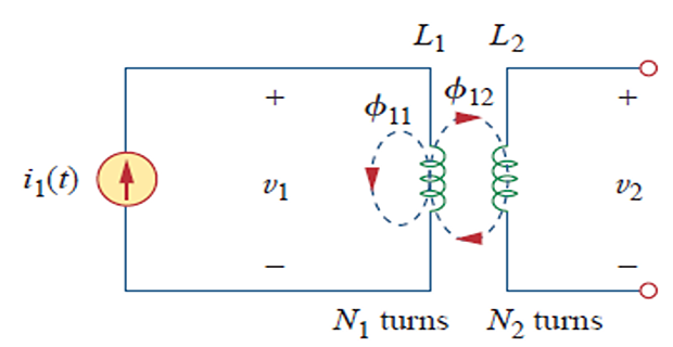
Two conditions for coupling to exist: the coils must be in close proximity, so that appreciable flux links both; and the circuits must be driven by time-varying sources, since a constant current produces no changing flux.
A point about signs. \(M\) is always a positive quantity, but the mutual voltage \(M\,di/dt\) may be positive or negative. For self-inductance the passive sign convention settles the polarity; for mutual inductance it cannot, because four terminals are involved and the coils' physical winding directions matter. Determining the polarity rigorously means examining the orientation of both windings and applying Lenz's law with the right-hand rule — which is exactly the tedious exercise the next section exists to avoid.
The Dot Convention
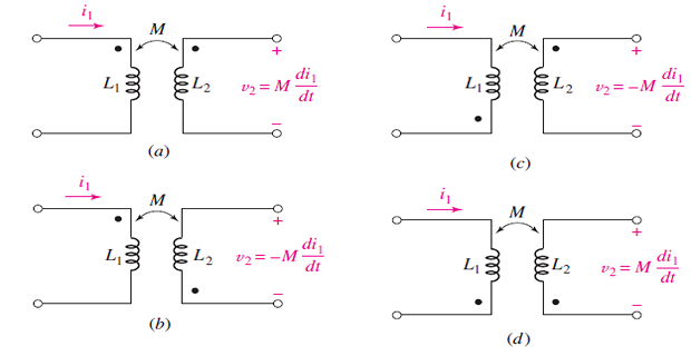
Rather than draw the winding direction of every coil, circuit diagrams mark one terminal of each coil with a dot. The dots encode the relative winding sense, and from them the sign of every mutual term follows mechanically.
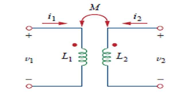
A current entering the dotted terminal of one coil produces an open-circuit voltage that is positive at the dotted terminal of the second coil.
Equivalently: a current entering the undotted terminal of one coil produces a voltage positive at the undotted terminal of the other.
The practical rule for writing equations is simply stated:
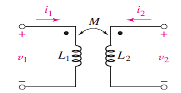
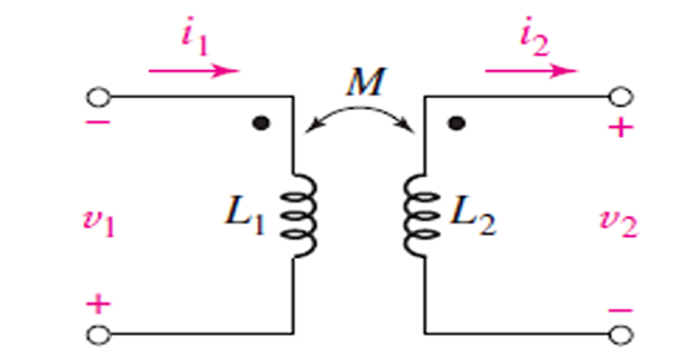
Note that only the relative positions of the dots matter. Moving both dots to the other terminals leaves every equation unchanged, because both mutual terms change sign together.
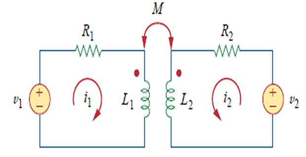
With resistance included and both currents entering their dots, the two loop equations become
Each equation has a self term involving its own current and a mutual term involving the other. In the frequency domain, replacing \(d/dt\) by \(j\omega\) as in Chapter 9:
The quantity \(j\omega M\) is the mutual impedance, in ohms. Note the symmetry of the coefficient matrix — the same \(j\omega M\) appears off-diagonal in both rows, which is the phasor statement of \(M_{12} = M_{21}\).
Series and Parallel Coupled Coils
Two coupled coils connected in series behave as a single inductor, but the value depends on how the coupling adds.
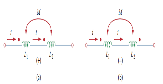
Series aiding — the current enters the dotted terminal of both coils, so the fluxes reinforce:
Series opposing — the current enters the dot of one and leaves the dot of the other, so the fluxes oppose:
The factor of 2 appears because each coil contributes a mutual term from the other's current, and both currents are the same in series.
This gives an elegant measurement method for \(M\), which is otherwise hard to determine directly. Measure the inductance both ways and subtract:
A single meter and one reversed connection suffice. The method also identifies which connection is aiding: the one giving the larger reading.
For coils in parallel the corresponding results are
with the upper sign for aiding and the lower for opposing. These arise less often, and when they do it is usually easier to convert to the T equivalent of Section 13.7 and combine in the ordinary way.
Problem. Two coils connected in series measure 19 H one way and 7 H with one coil's connections reversed. If \(L_{1} = 5~\mathrm{H}\), find \(M\), \(L_{2}\) and the coupling coefficient.
Solution. The larger reading is the aiding connection. Subtracting:
Adding the two readings instead eliminates \(M\):
The coupling coefficient follows from Section 13.5:
Since \(k < 0.5\) these coils are loosely coupled. Note that two simple inductance measurements have yielded all three parameters.
Energy and the Coupling Coefficient
To find the energy stored in a coupled pair, build the currents up one at a time and add the work done.
Step 1. With \(i_{2} = 0\), raise \(i_{1}\) from zero to \(I_{1}\). Only self-inductance is involved:
Step 2. Now hold \(i_{1}\) at \(I_{1}\) and raise \(i_{2}\) to \(I_{2}\). Two things happen at once: the second coil stores its own energy, and the source maintaining \(I_{1}\) must do work against the mutual voltage now appearing in coil 1:
Adding the two contributions gives the total stored energy:
The sign follows the dot convention exactly as before: positive if both currents enter their dotted terminals (or both leave), negative otherwise. Since \(I_{1}\) and \(I_{2}\) were arbitrary, the formula holds at every instant with lower-case currents.
The energy expression immediately answers a question that would otherwise be hard: how large can \(M\) be?
The circuit is passive, so the stored energy can never be negative. Taking the worst case — the negative sign — requires
Completing the square:
The squared term is never negative, so the inequality can only be guaranteed if the second term is non-negative for all currents:
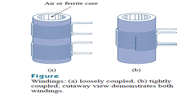
The mutual inductance can never exceed the geometric mean of the two self-inductances. The extent to which it approaches that limit is the coefficient of coupling:
\(k\) has a direct physical meaning: it is the fraction of the flux produced by one coil that links the other.
| Value of \(k\) | Description | Typical case |
|---|---|---|
| \(k = 1\) | perfectly coupled — all flux links both coils | an ideal transformer |
| \(k > 0.5\) | tightly coupled | iron-cored transformer, \(k \approx 0.99\) |
| \(k < 0.5\) | loosely coupled | air-cored coils, radio-frequency coupling |
| \(k = 0\) | no coupling | coils far apart or at right angles |
Coupling is improved by winding the coils on a common ferromagnetic core, which confines the flux and forces it to link both windings. It is reduced by separating the coils, or by orienting their axes at right angles so that one produces no flux through the other — a technique used deliberately to prevent unwanted coupling between adjacent components.
Problem. Two coils have \(L_{1} = 0.4~\mathrm{H}\) and \(L_{2} = 0.9~\mathrm{H}\) with a coupling coefficient of 0.6. Find \(M\), and the energy stored when \(I_{1} = 2~\mathrm{A}\) and \(I_{2} = 3~\mathrm{A}\), for both dot arrangements.
Solution.
The three energy terms:
If both currents enter their dots:
If one enters and the other leaves:
The same currents in the same coils store two and a half times as much energy in one arrangement as the other. This is why reversing a winding matters, and why the dots must be marked on the diagram.
The Linear Transformer
A linear transformer is a coupled pair in which the coils are wound on a magnetically linear core — air, plastic or ferrite — so that the flux is proportional to the current. Such transformers are common at radio frequencies, where iron would be far too lossy.
Take a source \(\mathbf{V}\) driving the primary through \(R_{1}\), with a load \(\mathbf{Z}_{L}\) on the secondary. The two mesh equations, with the mutual sign chosen by the dots, are
Solving the second for \(\mathbf{I}_{2}\) and substituting into the first gives the impedance the source actually sees:
The final term is the reflected impedance: the secondary circuit, seen from the primary, appears as an extra impedance in series with it. The secondary influences the primary without being connected to it. This is the whole point of the chapter, expressed in one equation.
Two observations. Because \(M\) appears squared, the reflected impedance does not depend on the dot placement — replacing \(M\) by \(-M\) changes nothing. And the reflected impedance is the secondary impedance inverted: a large secondary impedance reflects as a small addition, and a short-circuited secondary reflects the most.
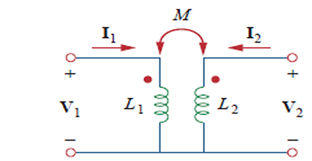
Problem. A linear transformer has, at the operating frequency, \(R_{1} = 4~\Omega\), \(\omega L_{1} = 8~\Omega\), \(\omega M = 6~\Omega\), \(R_{2} = 10~\Omega\) and \(\omega L_{2} = 12~\Omega\), with a load \(\mathbf{Z}_{L} = \left(6-j4\right)~\Omega\). A source \(\mathbf{V} = 50\angle 0^{\circ}~\mathrm{V}\) drives the primary. Find the coupling coefficient, the input impedance and both currents.
Solution. The coupling coefficient, using reactances since \(\omega\) cancels:
Tightly coupled. Now the total secondary impedance:
The reflected impedance:
Note that the reflected impedance is capacitive even though \(\mathbf{Z}_{22}\) is inductive — the reciprocal reverses the sign of the reactance. Adding to the primary:
and the secondary current from the second mesh equation:
Check: substituting into the first mesh equation, \(\left(4+j8\right)\mathbf{I}_{1} - j6\mathbf{I}_{2} = 50\angle 0^{\circ}\) \(\checkmark\). Note that current flows in the secondary although it is joined to the source by nothing at all.
Eliminating Mutual Inductance
Coupled circuits are awkward to analyse because the mutual terms couple the equations and the dots must be tracked. It is often easier to replace the coupled pair by an equivalent network of ordinary uncoupled inductors, and then use the methods of Chapter 10 without further thought.
The coupled pair is described by the matrix equation
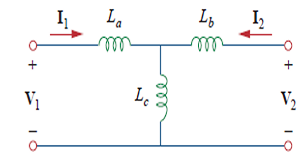
A three-element T network of uncoupled inductors \(L_{a}\), \(L_{b}\) (in the arms) and \(L_{c}\) (in the stem) has the matrix
Matching the two term by term gives the conversion:
Remarkably simple. Note that \(L_{a}\) or \(L_{b}\) may come out negative if \(M\) exceeds one of the self-inductances. A negative inductance cannot be built, but it is a perfectly valid element in an equivalent circuit and the mathematics handles it correctly.
Inverting the impedance matrix instead gives the Pi network equivalent:
The T form is usually preferred, being simpler to compute. Both assume the dots are in the standard position; if a dot is on the other terminal, replace \(M\) by \(-M\) throughout.
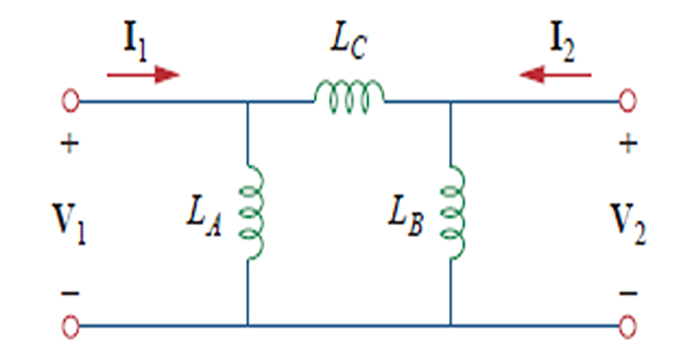
Problem. Find the T and Pi equivalents of the coupled pair from Example 13.1, where \(L_{1} = 5~\mathrm{H}\), \(L_{2} = 8~\mathrm{H}\) and \(M = 3~\mathrm{H}\).
T equivalent.
Pi equivalent. First the common numerator:
Verification. The T equivalent must reproduce the original impedance matrix, and the three entries check directly:
All three inductances here are positive because \(M\) is smaller than both self-inductances. Had \(M\) exceeded \(L_{1}\) or \(L_{2}\), one arm would have come out negative — see Practice Problem P13.4.
The Ideal Transformer
An ideal transformer is the limiting case in which the coupling is perfect and the windings are lossless. Formally it satisfies three conditions:
\(k = 1\) — perfect coupling, no leakage flux;
\(L_{1}, L_{2} \to \infty\) with their ratio fixed — infinite core permeability, so no magnetising current;
zero winding resistance and zero core loss.
Real iron-cored power transformers approach this closely: efficiencies above 98 % and coupling coefficients above 0.99 are routine, so the idealisation is a good one.
The turns ratio. With perfect coupling every turn of both windings links the same flux \(\phi\), so
Dividing one by the other, the flux cancels entirely:
The voltages are in the ratio of the turns. If \(n > 1\) the transformer steps down; if \(n < 1\) it steps up.
The current ratio. An ideal transformer is lossless, so all the power entering the primary leaves the secondary:
Voltage and current transform in opposite directions. A transformer that multiplies voltage by ten divides current by ten, and the product — the apparent power — is unchanged. Nothing is gained; the same power is repackaged at a different voltage. That is precisely what makes transmission economical: at ten times the voltage, one tenth of the current flows, and the \(I^{2}R\) losses fall by a factor of a hundred.
Dot placement. If both dots are at the top, the relations are as written. If one dot is moved, the ratio acquires a minus sign — the secondary voltage is inverted. This is worth checking before connecting transformers in parallel, where an inverted secondary produces a spectacular short circuit.
The most useful consequence follows by dividing the two relations. If a load \(\mathbf{Z}_{L}\) is connected across the secondary, the impedance seen at the primary is
This is the reflected or referred impedance for the ideal case, and note that it involves \(n\) squared. A transformer with a turns ratio of 10 makes a load appear a hundred times larger. The impedance angle is unchanged, since \(n^{2}\) is real and positive: a resistive load reflects as resistive, an inductive load as inductive.
This single relation is the basis of the impedance matching in the next section, and it is what finally completes the maximum-power-transfer problem left hanging in Chapter 11.
Problem. A 2400/240 V ideal transformer supplies a 12 \(\Omega\) resistive load on its secondary. Find the turns ratio, both currents, the impedance seen at the primary, and verify that power is conserved.
Solution. The turns ratio follows from the voltage ratio:
The secondary current is set by the load:
The reflected impedance:
Check by computing the primary current directly from it:
Power:
Identical, as they must be for a lossless device. Ten times the voltage, one tenth of the current, one hundred times the impedance, the same power.
Impedance Matching
Chapter 11 established that maximum average power is delivered when the load is the complex conjugate of the source impedance. It did not say what to do when the available load is simply the wrong value — which is nearly always the case.
The classic example is audio. An amplifier's output stage may have an internal resistance of a kilohm or more, while a loudspeaker is typically 4 or 8 \(\Omega\). Connected directly, almost all the power is dissipated inside the amplifier and the speaker receives a small fraction of what it could.
A transformer solves this exactly, because \(\mathbf{Z}_{\text{in}} = n^{2}\mathbf{Z}_{L}\) provides the missing ratio. Choosing
makes the load appear, at the source's terminals, to be exactly the impedance the source wants to see. The load itself is unchanged; only its apparent value is transformed.
Problem. An amplifier has a Thévenin resistance of 1250 \(\Omega\) and an open-circuit voltage of 100 V amplitude. It is to drive an 8 \(\Omega\) loudspeaker. Find the turns ratio for maximum power transfer, the power delivered, and compare with connecting the speaker directly.
Solution. The required turns ratio:
Checking: \(n^{2}Z_{L} = \left(156.25\right)\left(8\right) = 1250~\Omega\) \(\checkmark\) — a perfect match. The power delivered is then the maximum of Section 11.3:
Without the transformer, the 8 \(\Omega\) speaker connects directly across a 1250 \(\Omega\) source:
The matching transformer delivers nearly 40 times as much power — 1 W against 25 mW — from exactly the same amplifier and the same speaker. Nothing was added but a turns ratio.
This is why valve amplifiers, whose output stages have high impedance, invariably have a bulky output transformer, and why transistor amplifiers — with output impedances of a fraction of an ohm — do not need one.
Autotransformers and Three-Phase Transformers
An autotransformer has a single continuous winding, part of which is common to both primary and secondary. The output is taken from a tap. It therefore provides no electrical isolation — primary and secondary share a conductor — but it is smaller, cheaper and more efficient than a two-winding transformer of the same rating.
The reason is that only part of the power is transferred magnetically; the rest passes conductively through the shared winding, and that part requires no magnetic circuit at all. For a step-down autotransformer with ratio \(a = V_{1}/V_{2}\), the fraction transferred inductively is
The closer the ratio is to unity, the smaller this fraction and the greater the saving. Autotransformers are therefore used where a modest voltage change is needed — a variac, a motor starting autotransformer, or a transmission interconnection between 220 kV and 400 kV. They are not used where isolation is required for safety.
Problem. A 240/200 V step-down autotransformer supplies 5 kVA. Find the input and output currents, the current in the common winding, and compare the winding rating with that of an equivalent two-winding transformer.
Solution. The two line currents:
The common (lower) winding carries the difference, since part of the load current comes straight through from the input:
Now the ratings of the two winding sections:
Equal, as they always are. So windings rated at 833 VA handle a throughput of 5000 VA:
Confirming with the formula:
A six-fold saving in copper and core, for a transformer whose ratio is only 1.2:1. Had the ratio been 10:1 the saving factor would be only 1.11, which is why autotransformers are confined to modest ratios.
Chapter 12 assumed transformers throughout without saying how a three-phase supply is transformed. There are two approaches.
A bank of three single-phase transformers, one per phase, connected in Y or Δ on each side independently. This gives four combinations — Y–Y, Y–Δ, Δ–Y and Δ–Δ — chosen for the same reasons as the load connections of Section 12.3.
A single three-phase transformer with all six windings on one three-limb core. This is cheaper, smaller and more efficient than three separate units, and is the normal choice for new installations. A bank of three retains one advantage: if one unit fails, the other two can be reconnected in open delta to supply 58 % of the original rating until a replacement arrives.
The Δ–Y connection is the workhorse of distribution. The delta primary confines triplen harmonic currents to circulate within the closed loop rather than passing into the supply, while the star secondary provides the neutral that four-wire distribution requires. It also introduces a 30° phase shift between primary and secondary line voltages — harmless in itself, but it means transformers of different connection groups cannot be paralleled.
Practical Engineering Applications
The economic argument for transformers is worth stating numerically. Transmitting a fixed power \(P\) at voltage \(V\) requires current \(I = P/V\), and the line loss is \(I^{2}R = P^{2}R/V^{2}\). Losses fall as the square of the transmission voltage. Raising 11 kV to 220 kV — a factor of 20 — cuts the losses by a factor of 400.
This is the reason AC won the "war of the currents" in the 1890s. DC could not be transformed, so it had to be generated, transmitted and consumed at the same voltage, limiting distribution to a mile or two from the generating station. (Modern power electronics has since made HVDC transmission practical, and it now beats AC over very long distances and undersea — but only because semiconductor converters can do what no transformer can do for DC.)
Because primary and secondary share no conductor, a transformer provides galvanic isolation. An isolation transformer has a 1:1 ratio and exists purely for this property: with the secondary floating, touching either output terminal does not complete a circuit to earth, so a single accidental contact cannot deliver a shock. Medical equipment, laboratory test benches and equipment servicing all rely on this.
The same principle explains why an autotransformer must not be used where isolation is a safety requirement — its windings are connected, so the hazard passes straight through.
Measuring 400 kV or 2000 A directly is impractical and dangerous. A potential transformer (PT) steps the voltage down to a standard 110 V for the instrument, and a current transformer (CT) steps the current down to a standard 5 A or 1 A. Both exploit the same turns-ratio relations, and both isolate the operator from the high-voltage system.
A safety warning that follows directly from the theory. A current transformer's secondary must never be open-circuited while primary current flows. With no secondary current to oppose it, the primary current becomes entirely magnetising current, the core saturates hard, and the induced secondary voltage rises to lethal levels. CT secondaries are short-circuited before any instrument is disconnected — the opposite of the rule for potential transformers, whose secondaries must never be shorted.
SPICE describes coupling with a \(\texttt{K}\) statement naming two inductors and their coupling coefficient:
The simulator computes \(M = k\sqrt{L_{1}L_{2}}\) internally. Dot placement is implied by the order in which each inductor's nodes are listed, so reversing the two nodes of \(\texttt{L2}\) is equivalent to moving its dot — a convenient way to check both cases quickly.
Summary and Key Formulas
Mutual inductance couples two circuits through a shared magnetic field, with no conductor between them. It requires time-varying current.
The dot convention fixes the sign of every mutual term: current into a dot produces a voltage positive at the other dot.
Series coupled coils give \(L_{1}+L_{2}\pm2M\), and \(M\) can be measured from the difference of the two readings.
The stored energy is \(\tfrac{1}{2}L_{1}I_{1}^{2}+\tfrac{1}{2}L_{2}I_{2}^{2}\pm MI_{1}I_{2}\), and requiring it to be non-negative gives \(M \le \sqrt{L_{1}L_{2}}\).
The coupling coefficient \(k = M/\sqrt{L_{1}L_{2}}\) lies between 0 and 1, and is the fraction of flux that links both coils.
A linear transformer reflects its secondary into the primary as \(\omega^{2}M^{2}/\mathbf{Z}_{22}\), independent of dot placement.
Any coupled pair can be replaced by an uncoupled T network with \(L_{a} = L_{1}-M\), \(L_{b} = L_{2}-M\), \(L_{c} = M\).
An ideal transformer has \(V_{2}/V_{1} = 1/n\), \(I_{2}/I_{1} = n\) and \(\mathbf{Z}_{\text{in}} = n^{2}\mathbf{Z}_{L}\).
Impedance matching with \(n = \sqrt{R_{Th}/Z_{L}}\) completes the maximum-power problem of Chapter 11.
Autotransformers save material but provide no isolation; three-phase transformers use Y and Δ connections as in Chapter 12.
| Result | Formula | Notes |
|---|---|---|
| Mutual voltage | \(v_{2} = M\dfrac{di_{1}}{dt}\) | sign from the dots |
| Reciprocity | \(M_{12} = M_{21} = M\) | henrys |
| Coupled equations | \(\mathbf{V}_{1} = \left(R_{1}+j\omega L_{1}\right)\mathbf{I}_{1} \pm j\omega M\mathbf{I}_{2}\) | frequency domain |
| Series aiding | \(L = L_{1}+L_{2}+2M\) | both currents into dots |
| Series opposing | \(L = L_{1}+L_{2}-2M\) | |
| Measuring \(M\) | \(M = \dfrac{L_{\mathrm{aid}}-L_{\mathrm{opp}}}{4}\) | two measurements |
| Stored energy | \(w = \tfrac{1}{2}L_{1}i_{1}^{2}+\tfrac{1}{2}L_{2}i_{2}^{2}\pm Mi_{1}i_{2}\) | sign from the dots |
| Upper bound on \(M\) | \(M \le \sqrt{L_{1}L_{2}}\) | from passivity |
| Coupling coefficient | \(k = \dfrac{M}{\sqrt{L_{1}L_{2}}}\), \(0\le k\le1\) | \(k>0.5\) tight |
| Reflected impedance | \(\mathbf{Z}_{R} = \dfrac{\omega^{2}M^{2}}{R_{2}+j\omega L_{2}+\mathbf{Z}_{L}}\) | dot-independent |
| Linear transformer input | \(\mathbf{Z}_{\text{in}} = R_{1}+j\omega L_{1}+\mathbf{Z}_{R}\) | |
| T equivalent | \(L_{a}=L_{1}-M,\ L_{b}=L_{2}-M,\ L_{c}=M\) | no coupling |
| Pi equivalent | \(L_{C} = \dfrac{L_{1}L_{2}-M^{2}}{M}\) | and similarly \(L_{A}, L_{B}\) |
| Turns ratio | \(n = N_{1}/N_{2}\) | \(n>1\) step-down |
| Ideal voltage ratio | \(\mathbf{V}_{2}/\mathbf{V}_{1} = 1/n\) | |
| Ideal current ratio | \(\mathbf{I}_{2}/\mathbf{I}_{1} = n\) | opposite direction |
| Impedance transformation | \(\mathbf{Z}_{\text{in}} = n^{2}\mathbf{Z}_{L}\) | note the square |
| Matching ratio | \(n = \sqrt{R_{Th}/Z_{L}}\) | completes Chapter 11 |
| Autotransformer saving | \(\dfrac{S_{\text{total}}}{S_{\text{winding}}} = \dfrac{1}{1-V_{2}/V_{1}}\) | large for small ratios |
Common Mistakes
Ignoring the dots. The sign of every mutual term depends on them, and Example 13.2 showed the stored energy differing by a factor of 2.6 between the two arrangements.
Forgetting the factor of 2 in series connections. It is \(L_{1}+L_{2}\pm2M\), not \(\pm M\), because each coil sees the other's current.
Taking \(k > 1\). The coupling coefficient cannot exceed unity, so \(M\) can never exceed \(\sqrt{L_{1}L_{2}}\). If a problem's numbers give \(k > 1\), they are unphysical.
Using \(n\) instead of \(n^{2}\) for impedance. Voltage and current scale as \(n\); impedance scales as \(n^{2}\).
Inverting the turns ratio. With \(n = N_{1}/N_{2}\), the voltage ratio is \(V_{2}/V_{1} = 1/n\) but the current ratio is \(I_{2}/I_{1} = n\). Write down which is which before substituting.
Expecting the reflected impedance to depend on the dots. It contains \(M^{2}\), so it does not.
Rejecting a negative inductance in a T equivalent. It is legitimate in an equivalent circuit even though it cannot be built.
Assuming a transformer works on DC. Coupling requires \(d\phi/dt\). A transformer connected to DC presents only its winding resistance and burns out.
Believing a transformer gives power gain. It transforms voltage and current oppositely; the apparent power is unchanged, and a real one loses a little.
Open-circuiting a current transformer's secondary. Dangerous — the core saturates and the secondary voltage rises to lethal levels. Short it before disconnecting anything.
Chapter Review
Work these before opening the answers. State clearly which dot arrangement you have assumed wherever it matters.
P13.1 Two coils have \(L_{1} = 20~\mathrm{mH}\), \(L_{2} = 45~\mathrm{mH}\) and \(M = 24~\mathrm{mH}\). Find \(k\), and say whether the coupling is loose or tight.
Show answer
Since \(k > 0.5\) the coils are tightly coupled.\[\sqrt{L_{1}L_{2}} = \sqrt{\left(20\right)\left(45\right)} = 30~\mathrm{mH}, \qquad k = \frac{24}{30} = 0.8000\]P13.2 Two coupled coils in series measure 0.8 H aiding and 0.2 H opposing. Find \(M\) and \(L_{1}+L_{2}\).
Show answer
\[M = \frac{0.8-0.2}{4} = 0.15~\mathrm{H}, \qquad L_{1}+L_{2} = \frac{0.8+0.2}{2} = 0.5~\mathrm{H}\]P13.3 Coils with \(L_{1} = 2~\mathrm{H}\), \(L_{2} = 8~\mathrm{H}\) and \(k = 0.5\) carry \(I_{1} = 4~\mathrm{A}\) and \(I_{2} = 1~\mathrm{A}\), both entering their dots. Find the stored energy.
Show answer
\[M = 0.5\sqrt{16} = 2~\mathrm{H}\]If one current left its dot instead, \(w = 16+4-8 = 12.00~\mathrm{J}\).\[w = \tfrac{1}{2}\left(2\right)\left(16\right) + \tfrac{1}{2}\left(8\right)\left(1\right) + \left(2\right)\left(4\right)\left(1\right) = 16 + 4 + 8 = 28.00~\mathrm{J}\]P13.4 Find the T equivalent of a pair with \(L_{1} = 6~\mathrm{H}\), \(L_{2} = 4~\mathrm{H}\) and \(M = 5~\mathrm{H}\). Comment on the result.
Show answer
\(L_{b}\) is negative, which is perfectly acceptable in an equivalent circuit. Check the physics: \(k = 5/\sqrt{24} = 1.021 > 1\) — so these values are in fact unphysical, and no real coil pair could have them. A negative \(L_{b}\) with \(k \le 1\) would be legitimate.\[L_{a} = 6-5 = 1~\mathrm{H}, \qquad L_{b} = 4-5 = -1~\mathrm{H}, \qquad L_{c} = 5~\mathrm{H}\]P13.5 A linear transformer has \(\omega M = 8~\Omega\) and a total secondary impedance of \(\left(6+j8\right)~\Omega\). Find the reflected impedance.
Show answer
Capacitive, since the reciprocal reverses the sign of the reactance.\[\mathbf{Z}_{R} = \frac{64}{6+j8} = \frac{64\left(6-j8\right)}{100} = \left(3.84 - j5.12\right)~\Omega\]P13.6 An ideal transformer has 400 primary turns and 100 secondary turns. With 240 V on the primary and a 5 \(\Omega\) load, find \(V_{2}\), \(I_{2}\), \(I_{1}\) and \(Z_{\text{in}}\).
Show answer
\[n = \frac{400}{100} = 4, \qquad V_{2} = \frac{240}{4} = 60~\mathrm{V}\]\[I_{2} = \frac{60}{5} = 12~\mathrm{A}, \qquad I_{1} = \frac{12}{4} = 3~\mathrm{A}\]Check: \(240/80 = 3\) A \(\checkmark\), and \(P = 60(12) = 240(3) = 720\) W \(\checkmark\)\[Z_{\text{in}} = n^{2}Z_{L} = 16\left(5\right) = 80~\Omega\]P13.7 What turns ratio matches a 50 \(\Omega\) transmission line to a 450 \(\Omega\) antenna?
Show answer
Here the "source" is the 50 \(\Omega\) line and the "load" the antenna, so the transformer must make 450 \(\Omega\) look like 50 \(\Omega\):Check: \(n^{2}Z_{L} = (1/9)(450) = 50~\Omega\) \(\checkmark\)\[n = \sqrt{\frac{50}{450}} = \sqrt{0.1111} = 0.3333 \quad\text{(a 1:3 step-up)}\]P13.8 A 400/380 V autotransformer supplies 10 kVA. Find the saving factor over an equivalent two-winding transformer.
Show answer
The windings need be rated at only 500 VA to pass 10 kVA — an enormous saving, and exactly why autotransformers suit small ratios.\[\frac{S_{\text{total}}}{S_{\text{winding}}} = \frac{1}{1-380/400} = \frac{1}{0.05} = 20.00\]P13.9 A transmission line carries 100 MW. Compare the \(I^{2}R\) losses at 11 kV and at 220 kV.
Show answer
Since \(I = P/V\) and loss \(\propto I^{2}\):Four hundred times the loss at the lower voltage — the entire economic case for transformers.\[\frac{\text{loss at }11~\mathrm{kV}}{\text{loss at }220~\mathrm{kV}} = \left(\frac{220}{11}\right)^{2} = 20^{2} = 400\]P13.10 Two coils with \(L_{1} = L_{2} = L\) and coupling \(k\) are connected in series aiding. For what \(k\) is the total inductance four times \(L\)?
Show answer
Perfect coupling — and this is the maximum achievable, since \(k\) cannot exceed 1. Two identical perfectly coupled coils in series aiding behave as a single coil of \(4L\), which is the \(N^{2}\) law in disguise: doubling the turns quadruples the inductance.\[L_{\mathrm{eq}} = L+L+2kL = 2L\left(1+k\right) = 4L \;\Longrightarrow\; k = 1\]
MCQ 1. Mutual inductance requires:
(a) a conducting path between coils (b) time-varying current (c) DC excitation (d) equal turnsShow answer
(b) time-varying current. No conductor is needed, and DC produces no changing flux.MCQ 2. Two coupled coils in series opposing have an equivalent inductance of:
(a) \(L_{1}+L_{2}\) (b) \(L_{1}+L_{2}-M\) (c) \(L_{1}+L_{2}-2M\) (d) \(L_{1}+L_{2}+2M\)Show answer
(c). The factor of 2 arises because each coil sees the other's current.MCQ 3. The maximum possible value of \(M\) is:
(a) \(L_{1}+L_{2}\) (b) \(\sqrt{L_{1}L_{2}}\) (c) \(L_{1}L_{2}\) (d) unboundedShow answer
(b) the geometric mean, which follows from requiring the stored energy to be non-negative.MCQ 4. A coupling coefficient of 0.99 indicates:
(a) loose coupling (b) tight coupling (c) no coupling (d) an impossible valueShow answer
(b) tight coupling, typical of an iron-cored transformer.MCQ 5. The reflected impedance of a linear transformer:
(a) depends on dot placement (b) is independent of dot placement (c) equals \(\mathbf{Z}_{L}\) (d) is always inductiveShow answer
(b) independent, since it contains \(M^{2}\).MCQ 6. In the T equivalent of a coupled pair, the stem inductance \(L_{c}\) equals:
(a) \(L_{1}-M\) (b) \(L_{2}-M\) (c) \(M\) (d) \(L_{1}+L_{2}\)Show answer
(c) \(M\). The arms are \(L_{1}-M\) and \(L_{2}-M\).MCQ 7. An ideal transformer with \(n = 5\) and a 4 \(\Omega\) load presents a primary impedance of:
(a) 0.16 \(\Omega\) (b) 20 \(\Omega\) (c) 100 \(\Omega\) (d) 4 \(\Omega\)Show answer
(c) 100 \(\Omega\). \(n^{2}Z_{L} = 25(4)\). Option (b) wrongly uses \(n\) rather than \(n^{2}\).MCQ 8. An ideal transformer that steps voltage up by a factor of 4:
(a) steps current up by 4 (b) steps current down by 4 (c) leaves current unchanged (d) steps current down by 16Show answer
(b) down by 4. The apparent power is unchanged, so voltage and current transform oppositely.MCQ 9. An autotransformer:
(a) provides galvanic isolation (b) provides no isolation (c) works only on DC (d) has two separate windingsShow answer
(b) no isolation — its windings share a conductor, which is the price of its material saving.MCQ 10. A current transformer's secondary must never be:
(a) short-circuited (b) open-circuited (c) earthed (d) loadedShow answer
(b) open-circuited. The core saturates and the induced voltage becomes lethal. Note this is the opposite of the rule for a potential transformer.
A transformer transfers energy between two circuits that share no conductor. Trace the path the energy actually takes, and say what would happen if the core were removed.
The bound \(M \le \sqrt{L_{1}L_{2}}\) was derived from the requirement that stored energy be non-negative. Explain why a purely energetic argument can constrain a geometric property of two coils.
Impedance transforms as \(n^{2}\) while voltage and current transform as \(n\). Show that this is forced by the requirement that power be conserved.
A T equivalent may contain a negative inductance. Explain how this can be legitimate, and what physical constraint nonetheless limits which coupled pairs are realisable.
Example 13.6 obtained forty times more power from an unchanged amplifier and an unchanged speaker. Where did the extra power come from, and why is this not a violation of conservation of energy?
An autotransformer's saving is greatest when its ratio is closest to unity, yet a 1:1 autotransformer would be useless. Explain the trade-off, and say what a 1:1 two-winding transformer is nonetheless good for.
Part 2 has assumed throughout that circuits are driven at a single fixed frequency. Chapter 14 asks what happens as the frequency is varied, and the answer reshapes everything.
Since \(\mathbf{Z}_{L} = j\omega L\) rises with frequency while \(\mathbf{Z}_{C} = 1/j\omega C\) falls, every circuit containing both has one particular frequency at which they cancel exactly. At that resonant frequency the circuit becomes purely resistive and its response peaks sharply. The parameter \(\omega_{0} = 1/\sqrt{LC}\) defined back in Chapter 8 reappears as precisely this frequency, and the damping ratio becomes the quality factor that determines how sharp the peak is.
From resonance follow filters — circuits designed to pass some frequencies and reject others — and the Bode plot, the standard way of displaying how a circuit's gain and phase vary across many decades of frequency. Chapter 14 opens Part 3.