- Transform \(R\), \(L\) and \(C\) into their \(s\)-domain models, including initial conditions as sources.
- Apply the three-step procedure: transform the circuit, solve, invert.
- Solve integro-differential equations arising from circuit laws.
- Perform mesh and nodal analysis in the \(s\)-domain.
- Apply Thévenin's theorem and superposition to \(s\)-domain circuits.
- Obtain the transfer function and the impulse response of a network.
- Locate poles and zeros and draw a pole–zero diagram.
- Determine network stability from pole locations and by the Routh criterion.
- Write the state equations of a circuit and relate their eigenvalues to its poles.
Introduction
Chapter 15 developed the Laplace transform as mathematics. This chapter turns it on circuits, and the result is the most capable analysis method in the book.
The pattern will be familiar, because it is the third time we have used it. Chapter 2 established Ohm's law and Kirchhoff's laws for resistive circuits. Chapter 9 showed that both survive the phasor transform, so every DC technique carried over to AC with \(j\omega\) in place of real numbers. Now the same thing happens once more with \(s\) in place of \(j\omega\) — and this time nothing is left out.
Two things are genuinely new. First, initial conditions appear as independent sources in the transformed circuit, so a charged capacitor becomes a capacitor plus a voltage source and an energised inductor becomes an inductor plus a source. No separate natural-plus-forced decomposition is needed. Second, the transfer function \(H(s)\) and its poles turn out to govern everything at once: the transient shape, the frequency response, and whether the circuit is stable at all.
Setting \(s = j\omega\) recovers Part 2 entirely. The phasor method was never wrong — it was the special case in which the transient has died away and only one frequency is present.
Circuit Element Models
Each element's time-domain relation is transformed using the differentiation property of Section 15.4.
Resistor. Ohm's law contains no calculus, so it transforms unchanged:
Inductor. Applying \(\mathcal{L}\left[di/dt\right] = sI(s)-i(0^{-})\):
or, solving for the current instead,
Capacitor. Similarly, from \(i = C\,dv/dt\):
Read those equations as circuits. The inductor's voltage equation says: an impedance \(sL\) in series with a voltage source of value \(Li(0^{-})\). The current equation says the same thing in Norton form: an admittance \(1/sL\) in parallel with a current source \(i(0^{-})/s\). Either model may be used, and the choice is made to suit the analysis — series models for mesh analysis, parallel models for nodal.
| Element | Impedance \(Z(s)\) | Series model (for mesh) | Parallel model (for nodal) |
|---|---|---|---|
| Resistor | \(R\) | no initial condition | |
| Inductor | \(sL\) | \(sL\) with source \(Li(0^{-})\) | \(sL\) with source \(i(0^{-})/s\) |
| Capacitor | \(\dfrac{1}{sC}\) | \(\dfrac{1}{sC}\) with source \(\dfrac{v(0^{-})}{s}\) | \(\dfrac{1}{sC}\) with source \(Cv(0^{-})\) |
With zero initial conditions the sources vanish and only the impedances remain:
These are exactly the phasor impedances of Section 9.7 with \(j\omega \to s\). Everything that followed from them — series and parallel combination, voltage and current division, wye–delta — therefore holds unchanged.
The Analysis Procedure
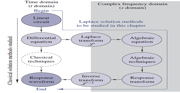
Every problem in this chapter follows three steps.
Transform the circuit from the time domain to the \(s\)-domain. Replace each source by its transform, each element by its impedance, and each initial condition by the appropriate source.
Solve the circuit by any technique — nodal, mesh, superposition, source transformation, Thévenin, Norton. The algebra is in \(s\); the methods are those of Chapters 3 and 4.
Invert the solution by partial fractions to return to the time domain.
The procedure is deliberately identical in shape to the phasor procedure of Section 10.2. What has changed is its reach: a step, a pulse, an exponential or a sinusoid can all be handled, and a circuit with stored energy needs no special treatment.
One point of technique. Because a transformed source such as \(1/s\) is itself a function of \(s\), the algebra produces fractions within fractions. Multiplying numerator and denominator by \(s\) at the earliest opportunity keeps the expressions manageable, and it is worth doing before rather than after collecting terms.
Integro-Differential Equations
Kirchhoff's laws applied to a circuit containing both an inductor and a capacitor produce an equation with both a derivative and an integral. The transform handles both at once, using \(\mathcal{L}\left[f'\right] = sF - f(0^{-})\) and \(\mathcal{L}\left[\int f\right] = F/s\).
Problem. Solve for the response \(y(t)\) in
Step 1 — transform each term. The derivative brings in the initial condition; the integral divides by \(s\); the step becomes \(1/s\):
Step 2 — solve algebraically. Multiply through by \(s\) and substitute \(y(0) = 2\):
Step 3 — invert.
Check. \(y(0) = -3+5 = 2\) \(\checkmark\). Note that the final value theorem gives \(\lim_{s\to0}sY(s) = 0\), and indeed both exponentials decay to zero — the integral term forces the response to settle at zero rather than at the step's value, because a non-zero \(y\) would make the integral grow without bound.
Mesh and Nodal Analysis
With impedances defined and Kirchhoff's laws intact, mesh and nodal analysis proceed exactly as in Chapters 3 and 10. The equations look the same; only the entries are functions of \(s\).
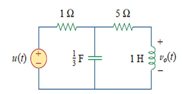
Problem. A source \(u(t)~\mathrm{V}\) drives mesh 1, which contains a 1 \(\Omega\) resistor and shares a \(\tfrac{1}{3}~\mathrm{F}\) capacitor with mesh 2. Mesh 2 contains the shared capacitor, a 5 \(\Omega\) resistor and a 1 H inductor, with \(v_{o}\) taken across the inductor. Find \(v_{o}(t)\), assuming zero initial conditions.
Step 1 — transform.
Step 2 — mesh equations.
Eliminating \(I_{1}\) gives \(I_{2} = 3/\left[s\left(s^{2}+8s+18\right)\right]\), and the output is the inductor voltage \(sI_{2}\):
Step 3 — invert by completing the square.
The complex poles at \(s = -4 \pm j\sqrt{2}\) produce a damped oscillation, exactly as Section 15.8 predicted. Note the sine numerator was arranged to equal \(\beta = \sqrt{2}\) before inverting — a step easily forgotten.
Circuits with Initial Conditions
Here the method shows its real advantage. A circuit with stored energy needs no separate transient analysis: the initial conditions simply appear as extra sources and the algebra proceeds unchanged.
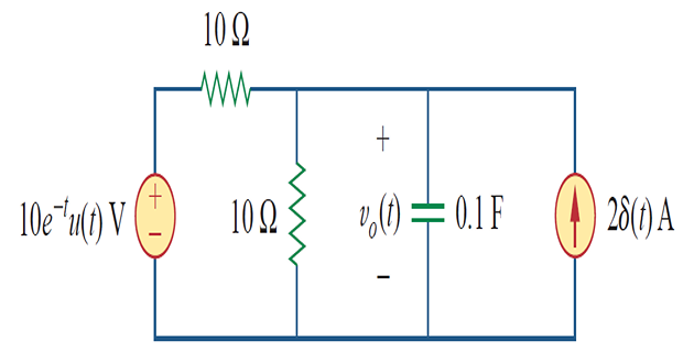
Problem. A source \(10e^{-t}u(t)~\mathrm{V}\) feeds a node through 10 \(\Omega\). A 2 A current source also feeds the node, which connects to ground through a second 10 \(\Omega\) resistor and a 0.1 F capacitor. The capacitor is initially charged to \(v_{o}(0) = 5~\mathrm{V}\). Find \(v_{o}(t)\).
Step 1 — transform, including the initial condition. The source becomes \(10/(s+1)\) and the capacitor becomes \(10/s\) in impedance. Using the parallel model, the charged capacitor contributes a current source
This is the key step, and it is worth pausing on: a capacitor charged to 5 V is equivalent to an uncharged capacitor in parallel with a 0.5 A current source. The stored energy has become an ordinary circuit element.
Step 2 — nodal analysis. KCL at the node, with both the 2 A source and the 0.5 A initial-condition source entering:
Multiplying by 10 and collecting terms in \(V_{o}\):
Step 3 — invert.
Check. \(v_{o}(0) = 10+15 = 25~\mathrm{V}\) — not 5 V. This is not an error: the initial capacitor voltage is 5 V, but \(v_{o}\) is the node voltage, which jumps at \(t=0\) because the current sources force current into the resistors instantaneously. Only capacitor voltage and inductor current are guaranteed continuous.
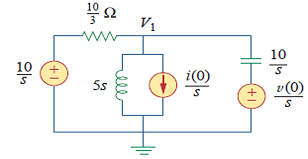
Problem. A circuit is driven by \(v_{s}(t) = 10u(t)~\mathrm{V}\) through a \(\tfrac{10}{3}~\Omega\) resistor. From the node, a 5 H inductor and a 0.1 F capacitor run to ground. The initial conditions are \(i_{L}(0) = -1~\mathrm{A}\) and \(v_{C}(0) = 5~\mathrm{V}\). Find \(v_{1}(t)\).
Solution. Both storage elements carry initial conditions, so both contribute sources. Writing KCL at the node with every branch accounted for:
The third term is the inductor's initial-condition current source \(i(0)/s = -1/s\), and the capacitor is modelled in series form with its \(v(0)/s\) source. Collecting:
Verify the partial fractions by recombining: \(35\left(s+2\right)-30\left(s+1\right) = 5s+40\) \(\checkmark\). At \(t=0\) the response is \(35-30 = 5~\mathrm{V}\), which here does match the capacitor's initial voltage because \(v_{1}\) is the capacitor voltage in this circuit.
Compare the effort with Chapter 8: a second-order circuit with two independent initial conditions and a step input, solved without ever classifying the damping, without finding a characteristic equation, and without fitting arbitrary constants.
Network Theorems in the s-Domain
Thévenin's and Norton's theorems, superposition and source transformation all apply in the \(s\)-domain, for the same reason they applied in the phasor domain: the circuit is linear and Kirchhoff's laws hold.
Note that \(Z_{Th}\) is now a function of \(s\) rather than a number — it may contain terms in \(s\) and \(1/s\), representing inductance and capacitance in the equivalent. A Thévenin equivalent in the \(s\)-domain is valid at all frequencies and for all time, unlike the phasor equivalent of Section 10.10 which held at one frequency only.
As in Chapter 4, when dependent sources are present the independent sources are deactivated but the dependent ones are kept, and \(Z_{Th}\) is found from the ratio above or by a test source.
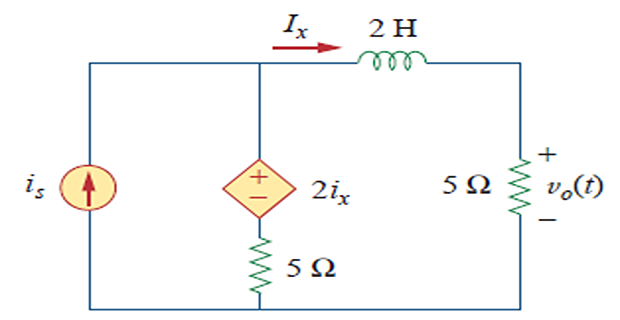
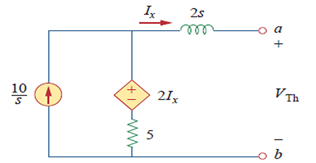
Problem. A network driven by \(i_{s} = 10u(t)~\mathrm{A}\) contains a 5 \(\Omega\) resistor, a 2 H inductor and a dependent source \(2I_{x}\), where \(I_{x}\) is the inductor current. Find \(V_{o}(s)\) across a 5 \(\Omega\) load using Thévenin's theorem, assuming no stored energy at \(t=0\).
Step 1 — open-circuit voltage. With the load removed, all the source current flows through the 5 \(\Omega\):
Step 2 — short-circuit current. With the terminals shorted, nodal analysis gives, using \(I_{x} = V_{1}/2s\):
Step 3 — the Thévenin impedance.
Note the form of the answer: \(2s+3\) is a 2 H inductor in series with a 3 \(\Omega\) resistor. The \(s\)-domain Thévenin impedance is itself a circuit.
Step 4 — the load voltage. Voltage division across the 5 \(\Omega\) load:
Inverting, since \(125/\left[s(s+4)\right] = 31.25/s - 31.25/(s+4)\):
A first-order step response — \(31.25\) V final value with a time constant of 0.25 s. The universal formula of Chapter 7 would have given the same answer, but only after separately identifying \(v(0)\), \(v(\infty)\) and \(\tau\); here it emerged from the algebra.
The Transfer Function
The transfer function of Chapter 14 returns, now as a function of \(s\) rather than \(\omega\):
defined for zero initial conditions, since it is meant to describe the network rather than its state. As before there are four kinds — voltage gain, current gain, transfer impedance and transfer admittance — depending on whether input and output are voltages or currents.
The impulse response. Consider the special case \(x(t) = \delta(t)\). Then \(X(s) = 1\) by Section 15.3, so
The impulse response is the inverse transform of the transfer function. They are the same object viewed in two domains, and this is why \(h(t)\) characterises the entire network: once it is known, the response to any input follows by convolution, or equivalently by multiplying transforms.
The relation \(Y(s) = H(s)X(s)\) is the convolution theorem of Section 15.9 read in the other direction. Convolution in time, multiplication in \(s\) — and the transfer function is what does the multiplying.
Problem. The output of a linear system is \(y(t) = 10e^{-t}\cos 4t\,u(t)\) when the input is \(x(t) = e^{-t}u(t)\). Determine the transfer function and the impulse response.
Solution. Transform both, using the frequency-shift property for the damped cosine:
The numerator and denominator have equal degree, so this is an improper fraction and long division is required before inverting — the point flagged in Section 15.6. Dividing:
Arranging the second term so its numerator is \(\beta = 4\):
The constant term inverts to an impulse, which is the signature of a transfer function whose numerator degree equals its denominator's. Physically it means the system passes an instantaneous component of the input straight through, unfiltered.
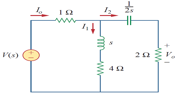
Problem. A current source \(I_{o}\) feeds a network in which a branch of impedance \(\left(s+4\right)\) is in parallel with a branch consisting of 2 \(\Omega\) in series with \(1/2s\). Find \(H(s) = V_{o}(s)/I_{o}(s)\), where \(V_{o}\) is taken across the 2 \(\Omega\).
Solution. Current division sends a fraction of \(I_{o}\) into the second branch:
Multiplying numerator and denominator by \(2s\) to clear the fraction within the fraction:
This is a transfer impedance, with units of ohms. Its zeros are at \(s = 0\) and \(s = -4\): at DC the transfer impedance vanishes, because the series capacitor blocks direct current entirely.
Poles, Zeros and the s-Plane
Any network function can be written as a ratio of polynomials, and then factored:
where \(K = a_{m}/b_{n}\) is the scale factor.
The roots of \(\mathbf{N}(s) = 0\) are the zeros, where the function vanishes. They are marked \(\bigcirc\) on a diagram.
The roots of \(\mathbf{D}(s) = 0\) are the poles, where the function becomes infinite. They are marked \(\times\).
Properties of the poles and zeros of a realisable network function:
If not repeated they are called simple; otherwise multiple.
Complex poles and zeros must occur in conjugate pairs, because the polynomial coefficients are real.
The real parts of all poles must be negative, and any pole on the \(j\omega\) axis must be simple.
The last property is the stability condition of the next section, stated in advance.
Why the diagram matters. Plotting the poles and zeros in the complex \(s\)-plane gives an immediate picture of the network's behaviour. A pole's real part sets an exponential decay rate; its imaginary part sets an oscillation frequency; a pole close to the \(j\omega\) axis decays slowly and dominates the response. The pole–zero diagram is used both in analysis and in synthesis, where a network is designed by first choosing where its poles should be.
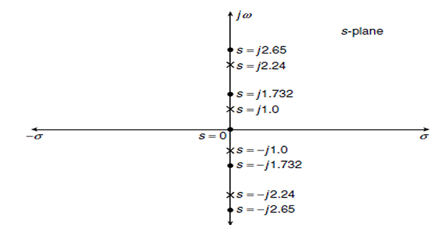
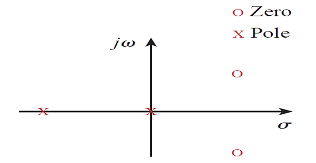
Problem. Draw the pole–zero diagram of the impedance function
Solution. Setting the numerator to zero gives the zeros, and the denominator the poles.
Two observations. Every pole and zero lies on the \(j\omega\) axis, with zero real part — the signature of a lossless network containing only inductors and capacitors, with no resistance to provide damping. And they alternate along the axis: zero at 0, pole at 1, zero at 1.732, pole at 2.236, zero at 2.646. This interlacing is a necessary property of any LC driving-point impedance, and it is the starting point for classical network synthesis.
Network Stability
A question that could not even be asked with phasors can now be answered precisely.
A network is stable if its response to a bounded input remains bounded. Since each pole \(p\) contributes a term \(e^{pt}\) to the impulse response, the condition is immediate:
A pole in the left half-plane gives a decaying exponential; a pole in the right half-plane gives one that grows without bound. The dividing line is the \(j\omega\) axis itself.
| Pole location | Contribution to \(h(t)\) | Classification |
|---|---|---|
| Left half-plane | decaying exponential | stable |
| Simple pole on \(j\omega\) axis | constant or sustained sinusoid | marginally stable |
| Repeated pole on \(j\omega\) axis | growing, e.g. \(t\sin\omega t\) | unstable |
| Right half-plane | growing exponential | unstable |
Note why a repeated pole on the axis is unstable while a simple one is not: the repetition introduces a factor of \(t\), as Section 15.7 showed, and \(t\sin\omega t\) grows without limit.
A passive RLC network is always stable, because its resistance always dissipates energy and pushes the poles into the left half-plane. A purely LC network is marginally stable — the case of Example 16.8. Instability requires an active element: an amplifier, a dependent source, or feedback. This is why oscillators are built with amplifiers, and why amplifier design is largely the art of keeping poles out of the right half-plane.
Factoring a high-order polynomial to find its roots is laborious, and often unnecessary — the question is usually not where the poles are but simply whether any lie in the right half-plane. The Routh–Hurwitz criterion answers that from the coefficients alone.
A necessary condition is easily stated: all coefficients of the denominator must be present and of the same sign. A missing or negative coefficient guarantees instability. It is not sufficient, however, and the full test uses an array. For the cubic \(s^{3}+a_{2}s^{2}+a_{1}s+a_{0}\):
The number of sign changes in the first column equals the number of right half-plane poles. For stability there must be none, which for the cubic requires all coefficients positive and \(a_{2}a_{1} > a_{0}\).
Problem. A network has the transfer function
Find the range of \(k\) for which the network is stable.
Solution. All coefficients are positive provided \(k > 0\), so the necessary condition gives no useful bound yet. Constructing the Routh array with \(a_{2} = 4\), \(a_{1} = k\), \(a_{0} = 10\):
For no sign changes in the first column, every entry must be positive:
Verification by direct root-finding. Computing the poles for several values of \(k\) confirms the boundary exactly:
| \(k\) | Poles | Result |
|---|---|---|
| 2 | \(-4.106\), \(+0.0530 \pm j1.560\) | unstable — pair in RHP |
| 2.5 | \(-4\), \(\pm j1.581\) | marginally stable — pair on the axis |
| 3 | \(-3.890\), \(-0.0552 \pm j1.602\) | stable |
| 5 | \(-3.395\), \(-0.3026 \pm j1.689\) | stable |
At exactly \(k = 2.5\) the complex pair sits precisely on the \(j\omega\) axis at \(\pm j1.581 = \pm j\sqrt{2.5}\), and the network oscillates indefinitely at that frequency without growing or decaying. This is exactly how an oscillator is designed: choose the gain that places a pole pair on the axis, and the circuit sustains an oscillation of its own accord. The Barkhausen criteria of Section 10.11 are this condition in another language.
Note also how the poles migrate: as \(k\) increases past 2.5 the complex pair moves steadily leftwards, so the response becomes better damped. Tracing that migration as a parameter varies is the root locus method of control engineering.
State Variables
All the methods so far produce a single high-order equation in one unknown. The state variable approach instead produces a set of first-order equations in several unknowns — a form far better suited to computation, and the standard language of modern control theory.
The state variables of a circuit are its capacitor voltages and inductor currents — precisely the continuous quantities identified in Chapter 6. They are chosen because they represent the circuit's stored energy, and hence its complete internal condition at any instant. Knowing them at \(t_{0}\), together with the inputs thereafter, determines the entire future.
The equations are written in matrix form:
where \(\mathbf{x}\) is the state vector, \(\mathbf{z}\) the input vector and \(\mathbf{y}\) the output. The first is the state equation, the second the output equation.
The procedure. Apply KCL at every node containing a capacitor to obtain \(dv/dt\), and KVL around every loop containing an inductor to obtain \(di/dt\). Then rearrange so that each derivative appears alone on the left.
Problem. Write the state equations of a series RLC circuit with \(R = 3~\Omega\), \(L = 1~\mathrm{H}\) and \(C = 0.5~\mathrm{F}\) driven by \(v_{s}\), and relate the eigenvalues of \(\mathbf{A}\) to the circuit's poles.
Step 1 — choose the state variables. The inductor current \(i\) and the capacitor voltage \(v\).
Step 2 — write one equation per element. KVL around the loop gives the inductor's derivative:
and the capacitor relation gives the other:
Step 3 — assemble in matrix form. Substituting \(R/L = 3\), \(1/L = 1\) and \(1/C = 2\):
Step 4 — find the eigenvalues. Setting \(\det\left(\mathbf{A}-\lambda\mathbf{I}\right) = 0\):
The eigenvalues are the poles. Check directly: the circuit's characteristic equation from Chapter 8 is \(s^{2}+\left(R/L\right)s+1/LC = s^{2}+3s+2\) — identical. The natural frequencies \(s_{1} = -1\) and \(s_{2} = -2\), the poles of \(H(s)\), and the eigenvalues of \(\mathbf{A}\) are three names for the same numbers.
Since both are real and distinct, the circuit is overdamped — a fact obtained here without ever computing \(\alpha\) or \(\omega_{0}\). And since both are negative, the circuit is stable, as any passive RLC circuit must be.
Why bother with the state form? It scales. A circuit with ten storage elements gives ten coupled first-order equations, which a computer integrates without difficulty, whereas the equivalent tenth-order differential equation is unmanageable. It also generalises to time-varying and non-linear systems, where transforms fail entirely.
Summary and Key Formulas
In the \(s\)-domain, \(Z_{R} = R\), \(Z_{L} = sL\) and \(Z_{C} = 1/sC\) — the phasor impedances with \(j\omega \to s\).
Initial conditions appear as independent sources: \(Li(0^{-})\) or \(i(0^{-})/s\) for an inductor, \(v(0^{-})/s\) or \(Cv(0^{-})\) for a capacitor.
The procedure is transform, solve, invert — with every technique from Chapters 3, 4 and 10 available unchanged.
Integro-differential equations become algebraic, with initial conditions built in.
The transfer function \(H(s) = Y(s)/X(s)\) assumes zero initial conditions, and \(h(t) = \mathcal{L}^{-1}\left[H(s)\right]\) is the impulse response.
Poles make a function infinite, zeros make it vanish; complex ones occur in conjugate pairs.
A network is stable if all poles lie in the left half-plane, marginally stable with simple poles on the \(j\omega\) axis, and unstable otherwise.
Passive RLC networks are always stable; instability requires an active element.
The Routh criterion tests stability from the coefficients, without factoring.
State variables are the capacitor voltages and inductor currents; the eigenvalues of \(\mathbf{A}\) are the network's poles.
| Result | Formula | Notes |
|---|---|---|
| Resistor | \(V(s) = RI(s)\) | unchanged |
| Inductor, series model | \(V(s) = sLI(s)-Li(0^{-})\) | for mesh analysis |
| Inductor, parallel model | \(I(s) = \dfrac{V(s)}{sL}+\dfrac{i(0^{-})}{s}\) | for nodal analysis |
| Capacitor, parallel model | \(I(s) = sCV(s)-Cv(0^{-})\) | for nodal analysis |
| Capacitor, series model | \(V(s) = \dfrac{I(s)}{sC}+\dfrac{v(0^{-})}{s}\) | for mesh analysis |
| Impedances | \(R\), \(sL\), \(1/sC\) | zero initial conditions |
| Thévenin impedance | \(Z_{Th}(s) = V_{oc}(s)/I_{sc}(s)\) | a function of \(s\) |
| Transfer function | \(H(s) = Y(s)/X(s)\) | zero initial conditions |
| Impulse response | \(h(t) = \mathcal{L}^{-1}\left[H(s)\right]\) | since \(\mathcal{L}[\delta] = 1\) |
| Any response | \(Y(s) = H(s)X(s)\) | convolution theorem |
| Factored form | \(H(s) = \dfrac{K\left(s-Z_{1}\right)\cdots}{\left(s-P_{1}\right)\cdots}\) | \(K = a_{m}/b_{n}\) |
| Stability | \(\mathrm{Re}\left(P_{i}\right) < 0\) for all \(i\) | left half-plane |
| Routh, cubic | \(a_{2}a_{1} > a_{0}\), all coefficients \(> 0\) | no sign changes |
| State equation | \(\dot{\mathbf{x}} = \mathbf{A}\mathbf{x}+\mathbf{B}\mathbf{z}\) | \(\mathbf{x}\) = \(v_{C}\), \(i_{L}\) |
| Output equation | \(\mathbf{y} = \mathbf{C}\mathbf{x}+\mathbf{D}\mathbf{z}\) | |
| Eigenvalues | \(\det\left(\mathbf{A}-\lambda\mathbf{I}\right) = 0\) | equal the poles |
Common Mistakes
Omitting the initial-condition sources. A charged capacitor is not just \(1/sC\) — it is \(1/sC\) plus a source. Forgetting the source silently assumes zero stored energy.
Mixing the series and parallel models within one element. Use \(Li(0^{-})\) or \(i(0^{-})/s\), never both.
Getting the polarity of the initial-condition source wrong. Derive it from the transformed equation rather than guessing; the sign follows from \(V(s) = sLI(s)-Li(0^{-})\).
Defining a transfer function for a circuit with stored energy. \(H(s)\) requires zero initial conditions; otherwise the ratio depends on the state as well as the network.
Inverting an improper fraction without dividing first. If the numerator degree is not less than the denominator's, long division is required — and the constant term inverts to an impulse, as in Example 16.6.
Expecting every node voltage to be continuous. Only capacitor voltages and inductor currents are. Example 16.3's node voltage jumps from 0 to 25 V.
Confusing poles with zeros on a diagram. Poles are crosses and make the function infinite; zeros are circles and make it vanish.
Judging stability from the numerator. Only the poles matter; zeros affect the shape of the response but never its stability.
Treating a simple \(j\omega\)-axis pole as unstable. It gives a sustained oscillation, which is marginally stable. A repeated axis pole is genuinely unstable.
Choosing the wrong state variables. They must be capacitor voltages and inductor currents — the continuous quantities — not resistor voltages or arbitrary node voltages.
Chapter Review
Work these before opening the answers. State initial conditions explicitly wherever they appear.
P16.1 Write the \(s\)-domain model of a 2 H inductor carrying an initial current of 3 A, in both series and parallel forms.
Show answer
Series: impedance \(2s\) with a voltage source \(Li(0^{-}) = 6~\mathrm{V}\).
Parallel: impedance \(2s\) with a current source \(i(0^{-})/s = 3/s\).P16.2 Solve \(\dfrac{dy}{dt}+4y+3\displaystyle\int_{0}^{t}y\,d\tau = 0\) with \(y(0) = 3\).
Show answer
\[sY-3+4Y+\frac{3}{s}Y = 0 \;\Longrightarrow\; Y\left(s^{2}+4s+3\right) = 3s\]\[Y = \frac{3s}{\left(s+1\right)\left(s+3\right)}, \qquad A = \frac{-3}{2} = -1.5, \qquad B = \frac{-9}{-2} = 4.5\]Check: \(y(0) = -1.5+4.5 = 3\) \(\checkmark\)\[y(t) = \left(-1.5e^{-t}+4.5e^{-3t}\right)u(t)\]P16.3 A series circuit of 4 \(\Omega\) and 0.5 H is driven by \(12u(t)~\mathrm{V}\) with \(i(0) = 0\). Find \(i(t)\) in the \(s\)-domain.
Show answer
\[I(s) = \frac{12/s}{4+0.5s} = \frac{24}{s\left(s+8\right)} = \frac{3}{s}-\frac{3}{s+8}\]Final value 3 A \(= 12/4\) \(\checkmark\), time constant \(L/R = 0.125~\mathrm{s}\) \(\checkmark\)\[i(t) = 3\left(1-e^{-8t}\right)u(t)~\mathrm{A}\]P16.4 Repeat P16.3 with \(i(0) = 2~\mathrm{A}\).
Show answer
The inductor now contributes a source \(Li(0) = 1~\mathrm{V}\):\[I(s) = \frac{12/s+1}{4+0.5s} = \frac{2\left(12+s\right)}{s\left(s+8\right)} = \frac{3}{s}-\frac{1}{s+8}\]Check: \(i(0) = 3-1 = 2\) \(\checkmark\) — the initial condition emerged from the algebra.\[i(t) = \left(3-e^{-8t}\right)u(t)~\mathrm{A}\]P16.5 Find the impulse response of a system with \(H(s) = \dfrac{5s}{s^{2}+6s+8}\).
Show answer
\[H(s) = \frac{5s}{\left(s+2\right)\left(s+4\right)}, \qquad A = \frac{-10}{2} = -5, \qquad B = \frac{-20}{-2} = 10\]\[h(t) = \left(-5e^{-2t}+10e^{-4t}\right)u(t)\]P16.6 Locate the poles and zeros of \(H(s) = \dfrac{4\left(s+3\right)}{s\left(s^{2}+2s+5\right)}\) and classify the network.
Show answer
Zero: \(s = -3\).
Poles: \(s = 0\) and, from \(s = \dfrac{-2\pm\sqrt{4-20}}{2}\), the pair \(s = -1 \pm j2\).
The complex pair is in the left half-plane, but the pole at the origin lies on the \(j\omega\) axis and is simple, so the network is marginally stable.P16.7 For what range of \(k\) is \(H(s) = \dfrac{1}{s^{3}+2s^{2}+ks+6}\) stable?
Show answer
Routh with \(a_{2} = 2\), \(a_{1} = k\), \(a_{0} = 6\):At \(k = 3\) the network is marginally stable, oscillating at \(\omega = \sqrt{3} = 1.732~\mathrm{rad/s}\).\[\frac{a_{2}a_{1}-a_{0}}{a_{2}} = \frac{2k-6}{2} > 0 \;\Longrightarrow\; k > 3\]P16.8 Write the state equations of a parallel RLC circuit with \(R = 1~\Omega\), \(L = 1~\mathrm{H}\), \(C = 1~\mathrm{F}\) driven by a current source \(i_{s}\).
Show answer
KCL at the node and the inductor relation give\[C\frac{dv}{dt} = i_{s}-\frac{v}{R}-i, \qquad L\frac{di}{dt} = v\]Eigenvalues: \(\lambda^{2}+\lambda+1 = 0\), giving \(\lambda = -0.5 \pm j0.866\) — complex, so the circuit is underdamped, and both have negative real part, so it is stable.\[\begin{bmatrix}\dot{v}\\\dot{i}\end{bmatrix} = \begin{bmatrix}-1 & -1\\1 & 0\end{bmatrix}\begin{bmatrix}v\\i\end{bmatrix}+\begin{bmatrix}1\\0\end{bmatrix}i_{s}\]P16.9 A system's step response is \(y(t) = \left(2-2e^{-5t}\right)u(t)\). Find \(H(s)\) and the impulse response.
Show answer
\[Y(s) = \frac{2}{s}-\frac{2}{s+5} = \frac{10}{s\left(s+5\right)}, \qquad X(s) = \frac{1}{s}\]Note that the impulse response is the derivative of the step response, since multiplying by \(s\) is differentiation.\[H(s) = \frac{Y}{X} = \frac{10}{s+5} \;\Longrightarrow\; h(t) = 10e^{-5t}u(t)\]P16.10 Explain why the transfer function of any passive RLC network can never have a pole in the right half-plane.
Show answer
A right half-plane pole gives a term \(e^{pt}\) with \(\mathrm{Re}(p) > 0\), so the response would grow without bound and the energy delivered to the network would increase indefinitely. A passive network contains no energy source, and its resistance can only dissipate — so unbounded growth is impossible. Instability therefore requires an active element capable of supplying energy.
MCQ 1. The \(s\)-domain impedance of a capacitor is:
(a) \(sC\) (b) \(1/sC\) (c) \(C/s\) (d) \(s/C\)Show answer
(b). Option (a) is the admittance.MCQ 2. An inductor with initial current \(i(0)\) is modelled in series form as \(sL\) with a source of value:
(a) \(i(0)/s\) (b) \(Li(0)\) (c) \(sLi(0)\) (d) \(i(0)\)Show answer
(b) \(Li(0)\), a voltage source. Option (a) is the parallel-model current source.MCQ 3. The transfer function is defined assuming:
(a) sinusoidal input (b) zero initial conditions (c) a stable network (d) unity gainShow answer
(b). Otherwise the ratio would depend on the stored energy as well as the network.MCQ 4. The impulse response of a network equals:
(a) \(H(s)\) (b) \(\mathcal{L}^{-1}\left[H(s)\right]\) (c) \(sH(s)\) (d) \(H(s)/s\)Show answer
(b), because \(\mathcal{L}\left[\delta(t)\right] = 1\), so \(Y(s) = H(s)\).MCQ 5. A network is stable if all poles lie:
(a) on the \(j\omega\) axis (b) in the right half-plane (c) in the left half-plane (d) at the originShow answer
(c). A negative real part gives a decaying exponential.MCQ 6. A simple pole on the \(j\omega\) axis makes a network:
(a) stable (b) marginally stable (c) unstable (d) overdampedShow answer
(b). It gives a sustained oscillation. A repeated axis pole would be unstable.MCQ 7. Stability is determined by a network function's:
(a) zeros (b) poles (c) scale factor (d) numerator degreeShow answer
(b) poles. Zeros shape the response but never destabilise it.MCQ 8. A passive RLC network is:
(a) always unstable (b) always stable (c) stable only if \(R\) is large (d) marginally stableShow answer
(b) always stable, since it has no energy source. Instability needs an active element.MCQ 9. The state variables of a circuit are the:
(a) node voltages (b) mesh currents (c) capacitor voltages and inductor currents (d) resistor voltagesShow answer
(c), because they are continuous and represent the stored energy.MCQ 10. The eigenvalues of the state matrix \(\mathbf{A}\) are the network's:
(a) zeros (b) poles (c) inputs (d) time constantsShow answer
(b) poles — equivalently its natural frequencies, as Example 16.10 shows.
Initial conditions appear as sources in the \(s\)-domain. Explain physically why stored energy should be equivalent to a source, and why the capacitor's source is a voltage while the inductor's series-model source is also a voltage.
The transfer function requires zero initial conditions, yet the analysis method handles non-zero ones easily. Reconcile these two statements.
A zero can lie anywhere in the \(s\)-plane without affecting stability, while a pole cannot. Explain the asymmetry.
In Example 16.3 the node voltage jumps from 0 to 25 V at \(t = 0\), although the capacitor voltage is 5 V throughout. Explain how both can be true.
Setting \(s = j\omega\) in \(H(s)\) recovers the frequency response of Chapter 14. What does this substitution mean physically, and what information is discarded by it?
A high-order circuit gives an unmanageable differential equation but a tractable set of state equations. Explain why the state formulation scales better, and name one class of system for which it works but transforms do not.
Every source in this book so far has been either DC, a single sinusoid, or a simple switching waveform. Real signals are none of these. A rectifier output, a square wave, a motor's current, a speech waveform — all are periodic or near-periodic but decidedly non-sinusoidal.
Chapter 17 shows that any periodic waveform, however jagged, can be expressed as a sum of sinusoids at multiples of its fundamental frequency. This is the Fourier series, and its consequence for circuit analysis is immediate: since the circuit is linear, its response to the whole waveform is the superposition of its responses to each harmonic — every one of which is an ordinary phasor problem from Part 2.
The promise made in Section 9.1 is finally kept. Understanding the response to one sinusoid really does mean understanding the response to everything, and Chapter 17 supplies the missing step.