Set 18 — Open-Circuit and Short-Circuit Tests
Set 17 assembled the equivalent circuit from parameters that were simply handed over. This set measures them. Two tests do the whole job: excite one winding at rated voltage with the other open, and the readings isolate the shunt branch; short one winding and raise the voltage only until rated current flows, and the readings isolate the series branch.
The arithmetic is short, so the difficulty lies elsewhere — in keeping track of which winding carried the instruments, and therefore which side every parameter belongs to. The set closes with Sumpner's back-to-back test, which delivers both sets of losses at once on two transformers running genuinely hot.
The open-circuit test gives the shunt branch. One winding — normally the LV, for instrument convenience — is excited at rated voltage while the other is left open. The current is the exciting current, so the wattmeter reads the iron loss:
\[ \cos\phi_0 = \frac{W_0}{V_0I_0}, \quad I_w = I_0\cos\phi_0, \quad I_\mu = I_0\sin\phi_0 \]\[ R_0 = \frac{V_0}{I_w}, \qquad X_0 = \frac{V_0}{I_\mu} \]The short-circuit test gives the series branch. One winding — normally the HV — is fed from a low voltage until rated current flows, the other being short-circuited. The flux is a few percent of normal, so the core loss is negligible and the wattmeter reads full-load copper loss:
\[ Z_{0k} = \frac{V_{sc}}{I_{sc}}, \qquad R_{0k} = \frac{W_{sc}}{I_{sc}^2}, \qquad X_{0k} = \sqrt{Z_{0k}^2 - R_{0k}^2} \]The subscript \(k\) is 1 or 2 according to which winding carried the instruments.
Refer whatever side the meters were on. With \(a = N_1/N_2\), series and shunt parameters both move by \(a^2\):
\[ R_{01} = a^2R_{02}, \qquad R_0^{(1)} = a^2R_0^{(2)} \]The two losses behave differently with load. Iron loss is fixed by the applied voltage; copper loss varies as the square of the load fraction \(x\):
\[ \eta = \frac{x S\cos\phi}{x S\cos\phi + P_i + x^2P_{cu,\text{fl}}} \]Maximum efficiency occurs where the two losses are equal:
\[ x^2P_{cu,\text{fl}} = P_i \;\Longrightarrow\; x = \sqrt{\frac{P_i}{P_{cu,\text{fl}}}}, \qquad S_{\max\eta} = xS \]Regulation follows from the short-circuit data alone:
\[ \%\text{reg} = \%R\cos\phi \pm \%X\sin\phi, \qquad \%R = \frac{I_2R_{02}}{V_2}\times100 \]Sumpner's test runs two identical transformers back to back. The primaries in parallel take only the combined iron loss; an auxiliary source injected into the opposed secondaries circulates rated current and supplies only the combined copper loss. Full-load heating is obtained at a fraction of full-load input.
In the no-load test of a single-phase transformer the following readings were obtained:
| Quantity | Reading |
|---|---|
| Primary voltage | 220 V |
| Secondary voltage | 110 V |
| Primary current | 0.5 A |
| Power input | 30 W |
The resistance of the primary winding is 0.6 Ω. Find
- the turns ratio
- the magnetising component of the no-load current
- the working (loss) component
- the iron loss
The turns ratio is the open-circuit voltage ratio. With no current flowing there is no impedance drop, so the terminal voltages are the induced EMFs:
This is the one measurement in the whole test set that is exact rather than inferred — which is why the open-circuit test is also the standard way of checking a nameplate ratio.
Extract the no-load power factor from the three meter readings:
Resolve the no-load current into its two components:
Separate the iron loss from the wattmeter reading. Strictly, the reading also contains the primary copper loss caused by the exciting current — normally ignored, and here is why:
The correction is 0.5% of the reading — smaller than the accuracy of the wattmeter itself. This is precisely why the open-circuit wattmeter is taken as reading iron loss directly.
The shunt-branch parameters follow, referred to the primary because that is the excited winding:
Obtain the equivalent circuit parameters of a 200/400 V, 50 Hz single-phase transformer from the following test data:
| Test | Voltage | Current | Power | Instruments on |
|---|---|---|---|---|
| Open circuit | 200 V | 0.7 A | 70 W | LV (200 V) side |
| Short circuit | 15 V | 10 A | 85 W | HV (400 V) side |
Hence calculate the secondary terminal voltage when the transformer delivers 5 kW at 0.8 power factor lagging, the primary voltage being held at 200 V.
Open-circuit test — the shunt branch. The instruments are on the 200 V winding, so everything obtained here is referred to the primary:
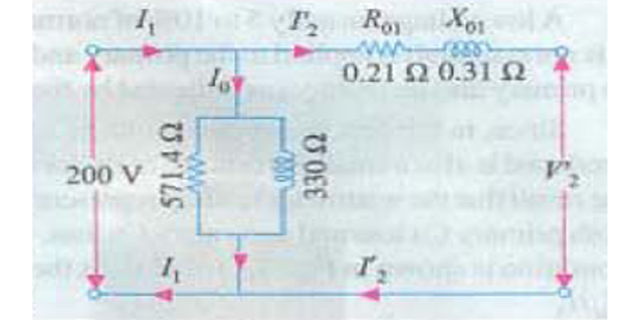
Short-circuit test — the series branch. Here the instruments have been placed on the secondary, that is on the high-voltage winding, while the low-voltage primary was short-circuited. Every parameter therefore comes out referred to the secondary:
Refer them to the primary as well, so that both tests describe the same circuit. This transformer steps up, so \(a < 1\) and the primary-side values are the smaller ones:
Find the secondary current at the stated load. The output is given in kilowatts, so the power factor must be divided out before the current can be found:
The 400 V used here is the no-load secondary voltage, since 200 V is applied to the primary and the ratio is 1:2. Using the as-yet-unknown loaded voltage would make the calculation circular; the small error this introduces is corrected below.
The total drop referred to the secondary, with the parameters obtained from the short-circuit test on that same winding:
Check the size of the neglected term. Solving the exact phasor relation \(|\bar{V}_2 + \bar{I}_2Z_{02}| = 400\) with \(\bar{I}_2 = 12.5 - j9.375\) gives \(V_2 = 377.7\ \text{V}\) — one tenth of a volt below the approximate answer, or 0.03%.
5.55% is a large regulation, and it comes almost entirely from \(X_{02}\): the reactive term contributes 11.6 V of the 22.2 V total at this power factor.
A 20 kVA, 2000/200 V, 50 Hz single-phase transformer gave the following test results:
| Test | Voltage | Current | Power | Instruments on |
|---|---|---|---|---|
| Open circuit | 200 V | 4.0 A | 120 W | LV (200 V) side |
| Short circuit | 70 V | 10 A | 420 W | HV (2000 V) side |
Determine
- \(R_0\) and \(X_0\), referred to the LV side and to the HV side
- \(R_{01}\), \(X_{01}\) and \(Z_{01}\)
- \(R_{02}\), \(X_{02}\) and \(Z_{02}\)
- the efficiency at full load, 0.8 power factor lagging
Confirm that the tests were run at the right operating points. This check takes ten seconds and catches most bad data:
The open-circuit test was at rated LV voltage (200 V) and the short-circuit test at rated HV current (10 A). Both are as they should be, so the iron loss is the true rated-voltage value and the copper loss is the true full-load value.
Open-circuit test. The exciting current is 4 A against a rated 100 A on that winding — 4%, which is normal:
Move the shunt branch to the HV side, where the short-circuit data already live:
A check that costs nothing: the iron loss computed on either side must agree. \(200^2/333.3 = 120\ \text{W}\) and \(2000^2/33\,330 = 120\ \text{W}\).
Short-circuit test — series parameters referred to the HV winding, since that is where the meters were:
The same parameters on the LV side, obtained by division rather than by repeating the work:
Efficiency at full load and 0.8 power factor. Both losses are now known at that operating point — the iron loss from the first test, the copper loss from the second:
Collect the equivalent circuit in one place. Six numbers describe the machine completely, and every one of them came from two meter readings and a stopwatch's worth of arithmetic:
| Parameter | Referred to HV (2000 V) | Referred to LV (200 V) |
|---|---|---|
| \(R\) series | 4.2 Ω | 0.042 Ω |
| \(X\) series | 5.6 Ω | 0.056 Ω |
| \(Z\) series | 7.0 Ω | 0.070 Ω |
| \(R_0\) | 33.3 kΩ | 333.3 Ω |
| \(X_0\) | 5057 Ω | 50.57 Ω |
| Losses | \(P_i = 120\ \text{W}\), \(P_{cu,\text{fl}} = 420\ \text{W}\) | |
A 10 kVA, 2000/400 V, 50 Hz single-phase transformer gave these results:
| Test | Voltage | Current | Power | Instruments on |
|---|---|---|---|---|
| Open circuit | 400 V | 1.0 A | 96 W | LV (400 V) side |
| Short circuit | 50 V | 5.0 A | 150 W | HV (2000 V) side |
Determine
- the percentage resistance, reactance and impedance
- the full-load regulation at 0.8 lagging, unity and 0.8 leading power factor
- the load at which the efficiency is a maximum, and that maximum efficiency at 0.8 power factor
- how the maximum compares with the full-load efficiency at the same power factor
Series parameters from the short-circuit test. The rated HV current is \(10\,000/2000 = 5\ \text{A}\), which is exactly the test current, so 150 W is the full-load copper loss:
Express them as percentages of rated volts, which is the form regulation wants:
A 2.5% impedance also says that a dead short on the secondary would draw \(100/2.5 = 40\) times rated current — the number a protection engineer takes from this test.
Regulation at the three power factors. Only the sign and size of the reactive term change:
| Load power factor | \(\%R\cos\phi\) | \(\pm\%X\sin\phi\) | Regulation |
|---|---|---|---|
| 0.8 lagging | 1.20% | +1.20% | 2.4% |
| Unity | 1.50% | 0 | 1.5% |
| 0.8 leading | 1.20% | −1.20% | 0% |
At 0.8 leading the two drops cancel exactly, because \(\%R/\%X = 1.5/2.0 = 0.75 = \tan(36.87^\circ)\). The terminal voltage at full load is then identical to its no-load value.
The load fraction for maximum efficiency is where the variable loss has grown to equal the fixed loss:
The maximum efficiency itself, at 0.8 power factor. At this load the copper loss has fallen to \(0.8^2 \times 150 = 96\ \text{W}\), equal to the iron loss as required:
Compare with full load at the same power factor:
Only 0.07 percentage points separate them. The efficiency curve is extremely flat near its peak, which is why designers place the maximum well below full load — around 75–85% for a distribution transformer that spends most of its life part-loaded.
Both tests on a 24 kVA, 2400/240 V, 50 Hz single-phase transformer were carried out with the instruments connected on the high-voltage winding:
| Test | Voltage | Current | Power | Condition of the LV winding |
|---|---|---|---|---|
| Open circuit | 2400 V | 0.5 A | 240 W | Open |
| Short circuit | 60 V | 10 A | 360 W | Short-circuited |
Find the complete equivalent circuit referred to the low-voltage side, and hence the secondary terminal voltage and percentage regulation at full load, 0.8 power factor lagging.
Note where every reading was taken before touching it. Both tests are on the HV winding, so both sets of parameters emerge referred to the HV side and both must later be divided by \(a^2\):
The short-circuit test was run at 10 A, which is rated HV current — so 360 W is the full-load copper loss and no scaling of the wattmeter reading is needed.
Open-circuit test, HV side. Exciting the HV winding is unusual and demands care: the current is only 0.5 A and the power factor 0.2, so a low-power-factor wattmeter is essential:
Refer the shunt branch to the LV side by dividing by \(a^2 = 100\):
The iron loss must be the same number whichever side it is computed on. If it is not, the referral went the wrong way — the commonest error in this type of problem, and one that this single line catches every time.
Short-circuit test, HV side:
Terminal voltage and regulation at full load, 0.8 lagging. All quantities are now on the LV side, so the calculation is a single line:
Alternative method — stay on the HV side throughout. The percentages are side-independent, so the same answer follows without ever referring anything:
Working in percentages sidesteps the referral entirely, which is why per-unit notation is the professional's default for any problem where the side of a measurement is in doubt.
Two identical 10 kVA, 500/250 V, 50 Hz single-phase transformers are tested back to back by Sumpner's method. Their primaries are connected in parallel across a 500 V supply and their secondaries in series opposition, with a low-voltage auxiliary source injected into the secondary loop. The readings are:
| Supply | Voltage | Current | Power |
|---|---|---|---|
| Primary side (both transformers) | 500 V | 2.0 A | 120 W |
| Auxiliary, in the secondary loop | 20 V | 40 A | 480 W |
Determine, for one transformer,
- the iron loss and the full-load copper loss
- \(R_{02}\), \(X_{02}\) and \(Z_{02}\)
- the efficiency at full load, 0.8 power factor lagging
- the load for maximum efficiency
Understand what each wattmeter is measuring. With the secondaries in opposition their induced EMFs cancel round the loop, so the 500 V supply drives no load current — it sees only two excited cores in parallel. The first wattmeter therefore reads the combined iron loss:
The 2 A drawn is the sum of two exciting currents, 1 A each against a rated primary current of \(10\,000/500 = 20\ \text{A}\) — 5%, exactly what an open-circuit test on a single unit would have shown.
The auxiliary source sees no EMF at all. It is injected into a loop whose net induced voltage is zero, so it needs only to overcome the impedance of the two secondary circuits. The current it drives is a genuine load current, circulating between the transformers, and the wattmeter reads the combined copper loss:
The circulating current is 40 A, which is exactly rated secondary current — so 240 W is the full-load copper loss and needs no scaling.
Halve the auxiliary voltage before using it. The 20 V is shared between two identical secondary circuits in series, so each transformer sees 10 V — this is the step the test is designed to catch:
The percentage values, which show this to be an entirely ordinary machine:
Regulation at 0.8 lagging would be \(2.4(0.8) + 3.2(0.6) = 3.84\%\).
Efficiency at full load, 0.8 power factor:
The load for maximum efficiency:
Why the test is worth the trouble. Both transformers are carrying rated current and rated flux, so both are heating exactly as they would on full load — yet the total input drawn from the two supplies is only:
Three percent of the apparent power that a real load bank would have demanded, because the useful power circulates between the two machines and only the losses are drawn from the mains. That is the whole idea of a back-to-back test, and it is the only practical way to run a temperature-rise test on a large transformer.
Key Formulas
| Quantity | Relation | Notes |
|---|---|---|
| Turns ratio | \(a = V_{oc,1}/V_{oc,2}\) | From the OC test — Problem 1 |
| No-load power factor | \(\cos\phi_0 = W_0/(V_0I_0)\) | Typically 0.1–0.3 |
| Exciting components | \(I_w = I_0\cos\phi_0\), \(I_\mu = I_0\sin\phi_0\) | In phase and quadrature |
| Shunt branch | \(R_0 = V_0/I_w\), \(X_0 = V_0/I_\mu\) | Referred to the excited winding |
| Iron loss | \(P_i = W_0 = V_0^2/R_0\) | Fixed by voltage, not load — Problem 3 |
| SC impedance | \(Z_{0k} = V_{sc}/I_{sc}\) | \(k\) = winding with the meters |
| SC resistance | \(R_{0k} = W_{sc}/I_{sc}^2\) | Full-load \(P_{cu}\) if \(I_{sc}\) is rated |
| SC reactance | \(X_{0k} = \sqrt{Z_{0k}^2 - R_{0k}^2}\) | Never \(Z-R\) — Problems 2–5 |
| Referral | \(R_{01} = a^2R_{02}\), \(R_0^{(1)} = a^2R_0^{(2)}\) | Series and shunt alike — Problem 5 |
| Percentage values | \(\%R = I R_{0k}/V \times 100\) | Side-independent — Problems 4, 5 |
| Regulation | \(\%\text{reg} = \%R\cos\phi \pm \%X\sin\phi\) | \(-\) for leading — Problems 4, 5 |
| Efficiency | \(\eta = \dfrac{xS\cos\phi}{xS\cos\phi + P_i + x^2P_{cu,\text{fl}}}\) | \(x\) = fraction of full load |
| Maximum efficiency | \(x = \sqrt{P_i/P_{cu,\text{fl}}}\) | Where the two losses are equal — Problems 4, 6 |
| Short-circuit current | \(I_{sc}/I_{\text{fl}} = 100/\%Z\) | Protection setting — Problem 4 |
| Sumpner: iron loss | \(P_i = W_1/2\) per transformer | Primary-side wattmeter — Problem 6 |
| Sumpner: copper loss | \(P_{cu} = W_2/2\), \(Z_{02} = (V_2/2)/I_2\) | Auxiliary voltage is shared — Problem 6 |
Common Mistakes
Forgetting which winding carried the instruments. \(V_{sc}/I_{sc}\) is \(Z_{02}\) when the meters are on the secondary and \(Z_{01}\) when they are on the primary; confusing the two is a factor of \(a^2\) — Problems 2 and 5.
Obtaining \(X\) by subtracting \(R\) from \(Z\). They combine in quadrature: \(\sqrt{7.0^2-4.2^2} = 5.6\), not \(7.0-4.2 = 2.8\) — Problem 3.
Taking the short-circuit wattmeter as full-load copper loss when the test current was not rated. The reading scales as the square of the current, so it must be multiplied by \((I_{\text{fl}}/I_{sc})^2\) first — checked explicitly in Problems 3, 4 and 5.
Attributing core loss to the short-circuit test. At 2.5% of rated voltage the flux, and with it the iron loss, is a fraction of a percent of normal — Problem 4.
Attributing copper loss to the open-circuit test. Only the exciting current flows, so \(I_0^2R_1\) was 0.15 W against a 30 W reading — Problem 1.
Using the loaded secondary voltage to find the load current before it has been computed. Use the no-load value; the resulting error is a fraction of a percent — Problem 2.
Adding the reactive term with a plus sign on a leading load. It reverses, and at 0.8 leading in Problem 4 it cancels the resistive drop completely.
Setting maximum efficiency at full load. It occurs at \(x = \sqrt{P_i/P_{cu}}\), which was 0.8 in Problem 4 and 0.5 in Problem 6 — never automatically 1.
Using the whole auxiliary voltage in Sumpner's test. Two secondaries share it, so each sees half; forgetting this doubles \(Z_{02}\) — Problem 6.
Forgetting to halve Sumpner's wattmeter readings. Both instruments measure the losses of two transformers — Problem 6.
Two wattmeter readings have now produced the entire equivalent circuit, and with it the two performance figures that matter commercially. Regulation appeared repeatedly above as a by-product of the short-circuit impedance — one line of arithmetic once \(\%R\) and \(\%X\) are known — and it always carried the same qualification: the answer depends on the load power factor as much as on the transformer.
That dependence deserves a set of its own. The approximate drop formula used here is accurate to a few hundredths of a percent at ordinary power factors, but it is an approximation, and it hides the geometry that explains why regulation can be negative, where the maximum lies, and what the exact phasor construction actually says.
Next: Set 19 — Voltage Regulation, where the drop formula is derived from the phasor diagram, the exact and approximate expressions are compared, and the power factor of maximum and of zero regulation is found in general.