By the end of this chapter you should be able to:
Classify materials as diamagnetic, paramagnetic, ferromagnetic or ferrimagnetic, and explain ferromagnetism in terms of domains.
Describe the shape of the B–H curve, name its regions, and explain the physical process occurring in each.
Show from tabulated data that \(\mu_r = B/\mu_0 H\) is not constant, and locate the maximum-permeability point.
Distinguish normal, initial, maximum and incremental permeability, and say which applies in a given situation.
Trace the full hysteresis loop point by point and account for every segment.
Define retentivity and coercivity, and interpret the loop area as energy loss per cycle per unit volume.
Choose between hard and soft magnetic materials for a stated application, and justify the choice quantitatively.
Solve the inverse problem for a gapped non-linear circuit using the air-gap line construction.
Introduction
Three chapters have now been built on a quantity quoted as a single number — the relative permeability \(\mu_r\) — and each of them has carried a warning that the number is a fiction. Chapter 2 flagged it, Chapter 3 showed that it makes the inverse problem deceptively easy, and Chapter 4 turned it into a virtue by demonstrating that a dominant air gap hides the fiction rather well. This chapter finally confronts it.
The truth is that a ferromagnetic material's permeability varies by a factor of five or more across its working range, and depends not only on the present field but on the material's history. Both facts follow from the same physical picture — the magnetic domain — and both have consequences that run through the rest of the book. The variation of \(\mu_r\) is why machine magnetisation curves bend over. The history dependence is why transformers get warm doing nothing, why a relay stays stuck after its coil is de-energised, and why permanent magnets exist at all.
The compensation for this loss of algebraic convenience is that the material can be characterised once, experimentally, and then used as a graph. Reading \(H\) off a curve is no harder than dividing by \(\mu_0\mu_r\), so the direct problem barely changes. The inverse problem does change, and Section 5-8 gives the elegant graphical construction that solves it — the same construction that will reappear in Chapter 9 to locate the operating point of a permanent magnet.
Classification of Magnetic Materials
Every material responds to a magnetic field to some degree. The response is measured by the relative permeability, and it separates materials into four useful classes.
| Class | \(\mu_r\) | Behaviour | Examples |
|---|---|---|---|
| Diamagnetic | slightly < 1 | Weakly repelled; opposes the applied field | Copper, silver, bismuth, water |
| Paramagnetic | slightly > 1 | Weakly attracted; effect vanishes without the field | Aluminium, platinum, oxygen |
| Ferromagnetic | hundreds to \(10^{5}\) | Strongly attracted; retains magnetisation | Iron, cobalt, nickel, silicon steel |
| Ferrimagnetic | hundreds to thousands | Like ferromagnetic but electrically insulating | Ferrites, magnetite |
For machine purposes only the last two matter. A diamagnetic or paramagnetic material differs from air by a few parts per million, so for every calculation in this book \(\mu_r = 1\) for copper, aluminium, insulation and air alike.
A ferromagnetic material is divided into microscopic regions called domains, each already magnetised to saturation by the quantum exchange interaction between neighbouring atoms. In an unmagnetised specimen the domains point in random directions and cancel. Applying a field does not magnetise the atoms — they are already magnetised — it merely reorganises the domains. That single idea explains the shape of the B–H curve, the existence of saturation, and the whole of hysteresis.
Two consequences of the domain picture deserve stating now:
Saturation is inevitable. Once every domain points along the field there is nothing left to align, and further increases in \(H\) add flux only at the rate free space would: \(\mathrm{d}B/\mathrm{d}H \to \mu_0\).
Ferromagnetism has a temperature limit. Above the Curie temperature thermal agitation destroys the domain structure and the material becomes merely paramagnetic. For iron this is 770 °C, for nickel 358 °C, for cobalt 1121 °C. It is far above any machine's operating temperature, but it is exploited in induction heating and in thermal cut-outs.
Formally, the total flux density is the sum of the free-space contribution and the material's own magnetisation \(M\):
where \(\chi_m = \mu_r - 1\) is the magnetic susceptibility. For iron \(M \gg H\), so essentially all the flux density comes from the material rather than from the applied field — which is exactly the point of using iron.
The Magnetisation or B–H Curve
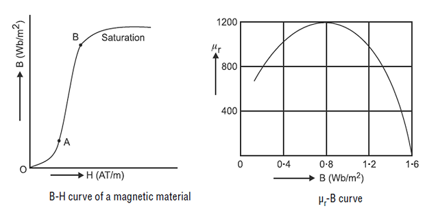
The B–H curve is simply a graph of flux density \(B\) against magnetising force \(H\) for a specimen taken from the unmagnetised state up to saturation. It is the single most useful piece of data about a magnetic material, and it is obtained by measurement, not by theory.
Two observations follow immediately from its shape:
The shape of the B–H curve is non-linear.
This indicates that \(\mu_r = B/\mu_0 H\) is not constant but varies, and that \(\mu_r\) depends largely on the value of \(B\).
By contrast, for a non-magnetic material the graph is a straight line through the origin, since \(B = \mu_0 H\) and therefore \(B \propto H\) exactly. Air, copper and insulation all lie on the same line, of slope \(\mu_0\) — imperceptibly shallow on any scale that shows iron properly.
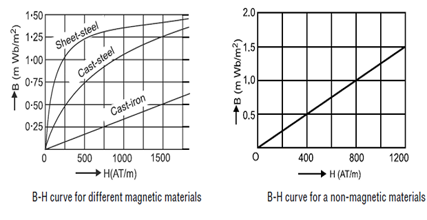
The following measured pairs are used throughout this chapter's examples and problems. Every value of \(\mu_r\) is computed from \(\mu_r = B/\mu_0 H\).
| \(H\) (AT/m) | 50 | 100 | 150 | 200 | 400 | 600 | 800 | 1000 | 1500 | 2000 | 3000 | 4000 | 6000 |
|---|---|---|---|---|---|---|---|---|---|---|---|---|---|
| \(B\) (T) | 0.08 | 0.20 | 0.32 | 0.45 | 0.80 | 1.00 | 1.11 | 1.18 | 1.30 | 1.36 | 1.44 | 1.49 | 1.55 |
| \(\mu_r\) | 1273 | 1592 | 1698 | 1790 | 1592 | 1326 | 1104 | 939 | 690 | 541 | 382 | 296 | 206 |
Read the bottom row carefully. Permeability rises to a maximum of about 1790 at \(H = 200\) AT/m and then falls steadily to 206 — a range of nearly nine to one. Quoting "\(\mu_r = 1200\)" for this material is meaningful only if you also say at what flux density.
Problem. Using Table 5.2, find the relative permeability at \(B = 0.45\) T, 1.00 T and 1.44 T. Comment on the consequences for the calculations of Chapters 2 to 4.
Solution. Read \(H\) for each \(B\) and apply \(\mu_r = B/\mu_0 H\).
Comment. The permeability at the top of the working range is less than a quarter of its maximum. A calculation performed at 0.45 T with \(\mu_r = 1790\) and then extrapolated to 1.44 T would underestimate the required mmf by a factor of nearly five.
This is exactly the trap flagged in Worked Example 3.5. The constant-\(\mu_r\) model is not wrong at a point — it is fitted at a point, and it fails as you move away from it. The safe practice is to treat any quoted \(\mu_r\) as a local tangent, valid over perhaps \(\pm 0.2\) T, and to use the curve whenever the flux density moves further than that.
Permeability Along the Curve
Because the curve is not a straight line, "the permeability" is ambiguous, and four distinct definitions are in use. Confusing them is a common and expensive error.
| Name | Definition | Where it is used |
|---|---|---|
| Normal (amplitude) | \(\mu = B/H\) — the chord from the origin | Ordinary DC magnetic-circuit calculations |
| Initial | \(\mu_i = \lim_{H\to 0} B/H\) | Instrument transformers, weak-signal work |
| Maximum | Largest value of \(B/H\) anywhere | Figure of merit when comparing materials |
| Differential / incremental | \(\mu_\Delta = \mathrm{d}B/\mathrm{d}H\) — the local slope | Small AC signal on a DC bias |
Consider a core biased to 1.30 T and carrying a small AC ripple. The normal permeability there is 690 (Table 5.2), and a designer who used that figure would predict a comfortable inductance. But the ripple sees only the local slope. From the table, between \(H = 1500\) and \(H = 2000\):
Ninety-five, against a normal permeability of 690 — a factor of more than seven. A choke designed on the normal figure would deliver about one-seventh of the intended AC inductance once the DC bias was applied. This is precisely why chokes carrying DC are gapped (Section 4-7): the gap's constant reluctance dominates, and the incremental behaviour becomes predictable.
Magnetic Hysteresis
Magnetic hysteresis is the phenomenon of the flux density \(B\) lagging behind the magnetising force \(H\). The word comes from the Greek hysterein, meaning to lag behind.
The lag arises because domain wall motion is not fully reversible. Walls become pinned on impurities, grain boundaries and crystal defects; freeing them costs energy, and when the field is removed they do not all return to where they started. The material therefore remembers.
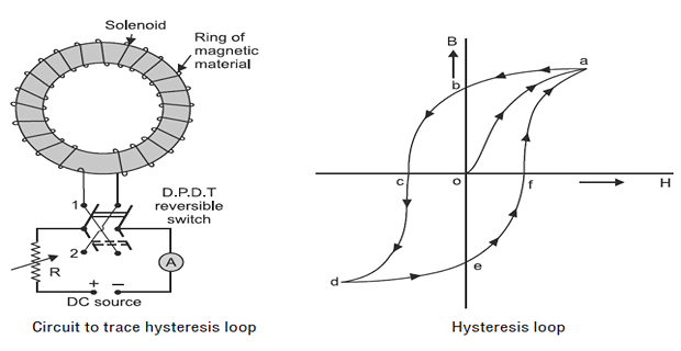
Imagine a ring specimen wound with a solenoid fed through a variable resistance \(R\) and a double-pole double-throw reversing switch. Starting from the completely unmagnetised state:
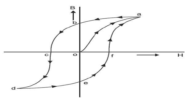
- o → a. \(H\) is increased gradually by increasing \(I\) in the solenoid (by decreasing \(R\)). \(B\) also increases until the saturation point a is reached. The curve so obtained is oa — the initial or virgin magnetisation curve, and the only time the specimen will ever travel this path.
- a → b. \(H\) is now gradually reduced to zero by decreasing \(I\) to zero. The flux density does not become zero; the curve obtained is ab. When \(H\) is zero, \(B\) still has the value ob.
- b → c. To demagnetise the specimen, \(H\) is reversed by reversing the direction of \(I\) — achieved by throwing the reversing switch to position 2. As \(H\) is increased in the reverse direction, \(B\) decreases and becomes zero, the curve following the path bc. The residual magnetism has been wiped off by applying the reverse field oc.
- c → d. To complete the loop, \(H\) is increased further in the reverse direction until saturation is reached at point d, the curve following cd.
- d → e. \(H\) is again reduced to zero and the curve follows de, where oe represents the residual magnetism in the reverse sense.
- e → f → a. \(H\) is then increased in the positive direction, by returning the reversing switch to position 1 and increasing the current. The curve follows efa and the loop is completed. Here of is the magnetising force needed to wipe off the residual magnetism oe.
Hence cf is the total coercive force required in one cycle of magnetisation to wipe off the residual magnetism, and the closed loop abcdefa so obtained is called the hysteresis loop.
Retentivity, Coercivity and Loop Area
Three quantities read off the loop characterise the material completely for engineering purposes.
The flux density ob retained when \(H\) has been reduced to zero is called the residual magnetism (or remanence, \(B_r\)). The power of the material to retain this residual magnetism is called its retentivity.
High retentivity is essential for permanent magnets, and useful in DC generators, where residual magnetism is what allows a self-excited machine to build up voltage at all (Chapter 28).
The value of \(H\) given by oc, required to wipe off the residual magnetism, is called the coercive force (or coercivity, \(H_c\)).
It measures how hard the material resists demagnetisation. It is the single figure that separates a permanent magnet from a transformer core — by a factor of about twenty thousand.
The energy supplied to a magnetic circuit per unit volume is \(\int H\,\mathrm{d}B\). Around a closed loop this integral does not vanish — it equals the enclosed area — and the difference is dissipated as heat in the material. A fat loop means a lossy material. Multiply by frequency and volume to get power:
When the loop is measured on a plotter or oscilloscope, the area is obtained in square centimetres of graph paper and converted using the two axis scales:
Chapter 6 takes this further, replacing the graphical area by Steinmetz's empirical law \(P_h = k_h f B_{\max}^{n} V\) with \(n\) between about 1.6 and 2.0, which is what designers actually use.
Problem. A hysteresis loop is plotted for a specimen to scales of 1 cm = 200 AT/m horizontally and 1 cm = 0.1 T vertically. The area enclosed is 42 cm². The core has a volume of 1200 cm³ and operates at 50 Hz. Find the hysteresis loss.
Energy per unit volume per cycle.
Volume in SI units.
Power loss.
Comment. Note that the energy per cycle is fixed by the material and the peak flux density alone; the power is proportional to frequency because the loop is traversed \(f\) times per second. Doubling the frequency doubles the hysteresis loss at the same \(B_{\max}\) — a fact that will matter greatly for the 400 Hz aircraft machines mentioned in Chapter 1, and which drives the choice of ferrite over steel at switching frequencies.
Hard and Soft Magnetic Materials
The loop shape divides magnetic materials into two families whose applications share almost nothing.
| Material | Type | \(B_r\) (T) | \(H_c\) (A/m) | Typical use |
|---|---|---|---|---|
| Silicon steel (CRGO) | Soft | ~1.4 | ~40 | Transformer and machine cores |
| Soft iron | Soft | ~1.3 | ~80 | Relay cores, pole pieces |
| Mn–Zn ferrite | Soft | ~0.4 | ~20 | High-frequency transformers |
| Permalloy | Soft | ~0.7 | ~4 | Instrument transformers, shielding |
| Alnico | Hard | ~1.25 | ~50 000 | Loudspeakers, older magnetos |
| Ferrite (ceramic) magnet | Hard | ~0.4 | ~200 000 | Low-cost motors, holding magnets |
| Neodymium (NdFeB) | Hard | ~1.25 | ~900 000 | PMSM and BLDC rotors, EV traction |
Problem. Estimate the hysteresis loss that a 0.02 m³ core would suffer at 50 Hz if built from (a) silicon steel with \(B_r = 1.4\) T, \(H_c = 40\) A/m, and (b) neodymium magnet material with \(B_r = 1.25\) T, \(H_c = 900\,000\) A/m. Approximate each loop as a rectangle of area \(4 B_r H_c\).
(a) Silicon steel.
(b) Neodymium.
Comment. Four and a half megawatts of heat in twenty litres of material. The core would not merely fail — it would vaporise within a fraction of a second. The rectangular approximation overstates a real loop by perhaps a factor of two or three, but no correction of that size affects the conclusion.
The two families are not interchangeable in either direction. A hard material is useless as a core because cycling it dissipates enormous energy; a soft material is useless as a magnet because the slightest opposing field wipes it clean. Note also that the silicon-steel figure, about 224 W for a 20-litre core, is realistic for a distribution transformer — which is why core loss is a headline specification and why grain-oriented steel commands its price.
Solving Circuits with the B–H Curve
With the curve in hand, the two problem types of Section 3-7 can finally be treated honestly.
The direct problem is barely changed. Given the flux, compute \(B = \Phi/A\), then read \(H\) from the curve instead of dividing by \(\mu_0\mu_r\), then form \(Hl\) as before. Everything else in Chapter 3 stands. Interpolate linearly between tabulated points.
The inverse problem needs a new idea. Given the mmf, the flux cannot be found directly because \(H\) in the iron depends on the very flux being sought. But for a circuit with an air gap there is an elegant construction that solves it in one step.
Write the mmf balance for iron plus gap, using \(H_g = B/\mu_0\):
This is a straight line in the \((H_i, B)\) plane — the same plane the material's curve is drawn in. Plot both; where they cross, both the material law and the circuit law are satisfied simultaneously. That intersection is the operating point.
The line is fixed by its two intercepts, which are worth memorising because they make it trivial to draw:
The flux density if the iron were perfect — infinite permeability, no mmf needed. An upper bound on what the circuit can achieve.
The field intensity if all the mmf were spent in the iron — that is, if there were no gap to cross.
Problem. A cast-steel ring of mean length 0.45 m and cross-section 5 cm² carries 600 turns. Using Table 5.2, find the current needed for a flux of 0.65 mWb (a) for the intact ring, and (b) after a 1 mm gap is cut.
(a) Intact ring.
From Table 5.2, \(B = 1.30\) T corresponds to \(H = 1500\) AT/m — read directly, no permeability required.
(b) With a 1 mm gap. The flux density is unchanged, so \(H_i\) is still 1500 AT/m, but the iron path shortens:
Comment. The gap takes 60.6 % of the mmf here, rather less than the 80 % typical of earlier examples, because the iron is being worked hard at 1.30 T where its permeability has fallen to 690. A saturated iron path competes with the gap on more equal terms — which is another way of saying that saturation costs ampere-turns just as an air gap does.
Problem. The gapped ring of Example 5.4 (iron 0.449 m, gap 1 mm, area 5 cm², 600 turns) is supplied with 2.0 A. Find the flux density and flux.
Step 1 — the available mmf.
Step 2 — the air-gap line.
Intercepts: \(B = 1.508\) T at \(H_i = 0\), and \(H_i = 1200/0.449 = 2673\) AT/m at \(B = 0\).
Step 3 — locate the intersection. Test the line against Table 5.2:
| \(H_i\) (AT/m) | 400 | 600 | 800 | 1000 |
|---|---|---|---|---|
| \(B\) from the curve | 0.80 | 1.00 | 1.11 | 1.18 |
| \(B\) from the line | 1.28 | 1.17 | 1.06 | 0.94 |
| Which is higher? | line | line | curve | curve |
The crossover lies between 600 and 800 AT/m. Interpolating the curve linearly there, \(B = 1.00 + 5.5\times10^{-4}(H_i - 600)\), and equating to the line:
Check. The two mmf drops must sum to 1200 AT:
Comment. At the operating point the effective \(\mu_r\) is \(1.084/(\mu_0 \times 752) = 1147\) — a value that could not have been guessed in advance, since it is neither the maximum 1790 nor the 690 that applies at 1.30 T. The construction finds the permeability as part of the answer rather than requiring it as an input. That is precisely why it works where algebra does not.
Applications
A transformer designer wants high saturation (to minimise core area), high permeability (to minimise magnetising current) and a narrow loop (to minimise loss). Grain-oriented silicon steel optimises all three along the rolling direction, which is why transformer cores are mitred so the flux always runs that way.
A shunt generator can only build up voltage because residual magnetism supplies a small initial flux. Without retentivity the machine would generate nothing at all. Chapter 28 shows how the field-resistance line intersects the magnetisation curve — the same construction as Section 5-8.
A BLDC or PMSM rotor needs the highest possible \(B_r\) together with a coercivity large enough to survive the demagnetising field of a fault current. The energy product \((BH)_{\max}\) is the standard figure of merit, and Chapter 9 uses the air-gap-line construction on the demagnetisation curve.
Storage media need a nearly rectangular loop: two stable remanent states with a sharp switching threshold. The same square-loop requirement drove ferrite core memory, and survives today in magnetic tape and hard-disk platters.
To erase a magnet or a machined steel part, apply an alternating field of decreasing amplitude. Each cycle traces a smaller loop, spiralling in towards the origin. Simply removing the field leaves \(B_r\) behind; simply applying \(-H_c\) leaves the material in an unstable state.
Heating a ferromagnetic workpiece past its Curie point makes it abruptly non-magnetic, collapsing the coupling. Self-regulating heaters exploit exactly this to hold a fixed temperature with no thermostat.
Summary and Key Formulas
Materials are diamagnetic, paramagnetic, ferromagnetic or ferrimagnetic. Only the last two matter for machines; everything else has \(\mu_r = 1\) for practical purposes.
Ferromagnetism is a domain phenomenon. Applying a field reorganises domains rather than magnetising atoms, which explains saturation, hysteresis and the Curie temperature.
The B–H curve is non-linear, so \(\mu_r = B/\mu_0 H\) is not constant. It rises to a maximum and then falls steeply — by nearly nine to one across the working range of Table 5.2.
For a non-magnetic material the curve is the straight line \(B = \mu_0 H\).
Incremental permeability \(\mathrm{d}B/\mathrm{d}H\) is far smaller than normal permeability on the flat part of the curve — a factor of seven in the example given — which is why DC-biased chokes must be gapped.
Hysteresis is the lagging of \(B\) behind \(H\). The loop abcdefa is traced by taking the specimen to saturation in both directions.
Retentivity \(B_r\) is the flux density remaining at \(H = 0\); coercivity \(H_c\) is the reverse field needed to remove it. Loop area is the energy lost per cubic metre per cycle.
Soft materials (narrow loop, low \(H_c\)) are for cores; hard materials (wide loop, high \(H_c\)) are for magnets. The two are never interchangeable.
The air-gap line \(B = (\mu_0/l_g)(NI - H_i l_i)\) intersects the B–H curve at the operating point, solving the inverse problem in one construction.
| Quantity | Formula | Notes |
|---|---|---|
| Magnetisation relation | \(B = \mu_0(H + M)\) | \(M\) is the material's magnetisation |
| Susceptibility | \(\chi_m = \mu_r - 1\) | tiny except for ferromagnets |
| Normal permeability | \(\mu_r = \dfrac{B}{\mu_0 H}\) | chord from the origin; varies with \(B\) |
| Incremental permeability | \(\mu_\Delta = \dfrac{\mathrm{d}B}{\mathrm{d}H}\) | local slope; use for AC on DC bias |
| Non-magnetic material | \(B = \mu_0 H\) | straight line, \(B \propto H\) |
| Saturation slope | \(\mathrm{d}B/\mathrm{d}H \to \mu_0\) | all domains aligned |
| Hysteresis energy | \(w_h = \oint H\,\mathrm{d}B\) | J/m³ per cycle = loop area |
| Loop area from a plot | \(w_h = A_{\mathrm{cm^2}} \times s_H \times s_B\) | \(s_H, s_B\) are the axis scales |
| Hysteresis power | \(P_h = w_h f V\) | proportional to frequency |
| Steinmetz law | \(P_h = k_h f B_{\max}^{n} V\) | \(n \approx 1.6\) to 2.0 — Chapter 6 |
| Air-gap line | \(B = \dfrac{\mu_0}{l_g}\left(NI - H_i l_i\right)\) | straight line on the B–H axes |
| Line intercepts | \(\dfrac{\mu_0 NI}{l_g}\) and \(\dfrac{NI}{l_i}\) | on the \(B\) and \(H\) axes |
| Line gradient | \(-\dfrac{\mu_0 l_i}{l_g}\) | shallower for a bigger gap |
Common Mistakes
Quoting a single \(\mu_r\) without saying at what flux density. It is a point on a curve, not a property of the material.
Using normal permeability where incremental permeability applies. For a small AC signal on a DC bias the local slope governs, and it may be seven times smaller.
Assuming maximum permeability occurs at maximum \(B\). It occurs quite low on the curve — at 0.45 T for the material in Table 5.2 — and falls steadily thereafter.
Confusing retentivity with coercivity. \(B_r\) is a flux density in teslas, read on the vertical axis; \(H_c\) is a field in A/m, read on the horizontal axis.
Treating the initial curve as part of the loop. The virgin curve oa is travelled once from the unmagnetised state and never again.
Forgetting to convert loop-area scales. Square centimetres of graph paper mean nothing until multiplied by both axis scales; the result is J/m³, not joules.
Forgetting the volume conversion. 1 cm³ = \(10^{-6}\) m³, not \(10^{-3}\). This slips a factor of a thousand into the loss.
Applying superposition to a saturating core. Non-linearity forbids it, as Chapter 2 warned. Two mmfs do not produce the sum of the fluxes they would produce separately.
Plotting the air-gap line against total \(H\) rather than \(H_i\) in the iron. The horizontal axis of the construction is the iron's field intensity; the gap's contribution is what the line's slope encodes.
Believing a gap prevents saturation. As Chapter 4 stressed, it does not — it merely makes it much harder for a given winding to reach saturation.
Chapter Review
Use Table 5.2 wherever B–H data is required, interpolating linearly between tabulated points.
P5.1 From Table 5.2, find \(\mu_r\) at \(B = 0.80\) T and at \(B = 1.49\) T, and state the ratio.
Show answer
A ratio of 5.37 to 1. Driving the core from 0.80 T to 1.49 T — less than double the flux density — costs ten times the magnetising force.\[\mu_r\big|_{0.80} = \frac{0.80}{(4\pi\times10^{-7})(400)} = 1592, \qquad \mu_r\big|_{1.49} = \frac{1.49}{(4\pi\times10^{-7})(4000)} = 296\]P5.2 A cast-steel ring of mean length 0.30 m and area 4 cm² carries 500 turns. Find the current for a flux of 0.48 mWb.
Show answer
Interpolating between \((1000, 1.18)\) and \((1500, 1.30)\):\[B = \frac{0.48\times10^{-3}}{4\times10^{-4}} = 1.20~\mathrm{T}\]\[H = 1000 + \frac{1.20-1.18}{1.30-1.18}(500) = 1000 + 83 = 1083~\mathrm{AT/m}\]\[NI = (1083)(0.30) = 325~\mathrm{AT} \quad\Longrightarrow\quad I = 0.650~\mathrm{A}\]P5.3 A 0.8 mm gap is cut in the ring of P5.2. Find the new current for the same flux, and the mmf split.
Show answer
Iron path \(0.30 - 0.0008 = 0.2992\) m, \(H_i\) still 1083 AT/m:\[\mathcal{F}_i = (1083)(0.2992) = 324~\mathrm{AT}\]\[H_g = \frac{1.20}{4\pi\times10^{-7}} = 9.549\times10^{5}, \qquad \mathcal{F}_g = (9.549\times10^{5})(0.0008) = 764~\mathrm{AT}\]The gap takes 70.2 % of the mmf. Check by the rule of thumb: \(800(1.20)(0.8) = 768\) AT \(\checkmark\)\[NI = 324 + 764 = 1088~\mathrm{AT} \quad\Longrightarrow\quad I = 2.176~\mathrm{A}\]P5.4 A circuit has an iron path of 0.40 m and a gap of 1.2 mm, excited by 1500 AT. Find the two intercepts of the air-gap line.
Show answer
\[B\big|_{H_i=0} = \frac{\mu_0 NI}{l_g} = \frac{(4\pi\times10^{-7})(1500)}{0.0012} = 1.571~\mathrm{T}\]The B-intercept of 1.571 T exceeds the material's saturation, which tells you at once that the operating point will lie well down the line, on the curved part of the characteristic.\[H_i\big|_{B=0} = \frac{NI}{l_i} = \frac{1500}{0.40} = 3750~\mathrm{AT/m}\]P5.5 A hysteresis loop is plotted to scales 1 cm = 250 AT/m and 1 cm = 0.08 T, enclosing 36 cm². The core volume is 900 cm³ and the frequency 60 Hz. Find the hysteresis loss.
Show answer
\[w_h = (36)(250)(0.08) = 720~\mathrm{J/m^{3}\ per\ cycle}\]\[P_h = (720)(60)(900\times10^{-6}) = 38.9~\mathrm{W}\]P5.6 On a hysteresis loop, which axis carries retentivity and which carries coercivity, and what are their units?
Show answer
Retentivity \(B_r\) is the intercept on the vertical (\(B\)) axis, in teslas — the flux density surviving at \(H = 0\).
Coercivity \(H_c\) is the intercept on the horizontal (\(H\)) axis, in A/m — the reverse field needed to drive \(B\) to zero.
A useful mnemonic: retentivity is what the material keeps; coercivity is what it takes to coerce it back.P5.7 A core has a hysteresis loss of 80 W at 50 Hz and 1.1 T. Anticipating Chapter 6, estimate the loss at 60 Hz and 1.2 T, taking the Steinmetz exponent as 1.7.
Show answer
Since \(P_h \propto f B_{\max}^{n}\):\[\frac{P_2}{P_1} = \frac{60}{50}\left(\frac{1.2}{1.1}\right)^{1.7} = (1.20)(1.1594) = 1.391\]A 20 % rise in frequency and a 9 % rise in flux density together add 39 % to the loss — the flux density term is the more punishing of the two.\[P_2 = (80)(1.391) = 111~\mathrm{W}\]P5.8 An induction-heated steel billet is raised past 770 °C. Describe what happens to the coupling and why.
Show answer
770 °C is the Curie temperature of iron. Above it, thermal agitation destroys the domain structure and the steel becomes merely paramagnetic, with \(\mu_r \approx 1\). The reluctance of the workpiece rises by three orders of magnitude, the coupling collapses, and the heating rate falls abruptly. Self-regulating induction heaters and Curie-point thermostats exploit exactly this transition.P5.9 A designer needs a material for (a) a 50 Hz transformer core, (b) a BLDC rotor magnet, (c) a magnetic shield for a sensitive instrument. Choose from Table 5.4 and justify each.
Show answer
(a) Silicon steel (CRGO) — narrow loop for low hysteresis loss, high saturation to keep the core small, and laminated to control eddy currents.
(b) Neodymium — the highest \(B_r\) combined with a coercivity high enough to survive the demagnetising field of a fault current.
(c) Permalloy — its very high initial permeability offers the low-reluctance bypass a shield needs, and its tiny \(H_c\) means it does not retain magnetisation and disturb the instrument.P5.10 A core is biased at \(H = 3000\) AT/m and carries a small AC ripple. Using Table 5.2, find the incremental relative permeability and compare it with the normal value.
Show answer
Between \(H = 3000\) and \(H = 4000\):The normal permeability at that point is 382, so the incremental value is smaller by a factor of 9.6. Deep in saturation the core has become almost as poor as air for small signals — which is the whole reason saturable reactors and magnetic amplifiers work.\[\mu_\Delta = \frac{1.49-1.44}{4000-3000} = 5.0\times10^{-5}~\mathrm{H/m} \quad\Longrightarrow\quad \mu_{r\Delta} = \frac{5.0\times10^{-5}}{4\pi\times10^{-7}} = 39.8\]
MCQ 1. The B–H curve of a non-magnetic material is:
(a) a saturating curve (b) a straight line through the origin (c) a closed loop (d) a hyperbolaShow answer
(b) a straight line through the origin, since \(B = \mu_0 H\) exactly and \(B \propto H\).MCQ 2. Relative permeability of a ferromagnetic material is:
(a) constant (b) proportional to \(H\) (c) variable, depending largely on \(B\) (d) always unityShow answer
(c) variable, depending largely on \(B\). It rises to a maximum and then falls steeply towards saturation.MCQ 3. Hysteresis means that:
(a) \(H\) lags \(B\) (b) \(B\) lags \(H\) (c) both are in phase (d) neither variesShow answer
(b) \(B\) lags \(H\). From the Greek hysterein, to lag behind.MCQ 4. The flux density remaining when \(H\) is reduced to zero is called:
(a) coercivity (b) residual magnetism (c) saturation (d) susceptibilityShow answer
(b) residual magnetism (remanence). The material's ability to retain it is its retentivity.MCQ 5. The area of a hysteresis loop represents:
(a) power loss per second (b) energy loss per cubic metre per cycle (c) stored energy (d) permeabilityShow answer
(b) energy loss per cubic metre per cycle. Multiply by \(f\) and \(V\) to obtain power.MCQ 6. A material suitable for a permanent magnet has:
(a) low \(H_c\), narrow loop (b) high \(H_c\), wide loop (c) high \(\mu_r\), no loop (d) zero \(B_r\)Show answer
(b) high \(H_c\), wide loop — a hard material, which resists demagnetisation.MCQ 7. Above the Curie temperature a ferromagnetic material becomes:
(a) diamagnetic (b) paramagnetic (c) superconducting (d) more permeableShow answer
(b) paramagnetic. Thermal agitation destroys the domain structure, and \(\mu_r\) falls to nearly 1.MCQ 8. Deep in saturation, \(\mathrm{d}B/\mathrm{d}H\) approaches:
(a) zero (b) \(\mu_0\) (c) \(\mu_0\mu_r\) (d) infinityShow answer
(b) \(\mu_0\). All domains are aligned, so further flux is added only as free space would add it.MCQ 9. The air-gap line is plotted on the same axes as the B–H curve because:
(a) it is a material property (b) their intersection satisfies both the material law and the circuit law (c) it measures loss (d) it is required by conventionShow answer
(b) their intersection satisfies both laws simultaneously — which is exactly what the operating point means.MCQ 10. Ferrites are preferred over laminated steel at high frequency because they are:
(a) more permeable (b) cheaper (c) electrical insulators (d) able to saturate at higher \(B\)Show answer
(c) electrical insulators. Their enormous resistivity suppresses eddy currents, which otherwise dominate at high frequency. Their permeability and saturation density are both lower than steel's.
Explain how the domain picture accounts for all three of saturation, hysteresis and the Curie temperature.
Maximum permeability occurs well below saturation. Explain why, in terms of what the domains are doing in each region of the curve.
Why is it meaningless to quote a relative permeability without also quoting a flux density? Give a numerical illustration from Table 5.2.
A choke carrying DC is found to have far less AC inductance than its designer expected. Diagnose the error and state the remedy.
The initial magnetisation curve is travelled only once. What must be done to a specimen before it can be travelled again, and why does simply switching off the current not suffice?
Silicon steel and neodymium have almost the same remanence but coercivities differing by twenty thousand times. Explain what physical property differs, and why that makes one a core material and the other a magnet.
Explain why the air-gap line construction succeeds where direct algebra fails, and identify what the intersection determines that could not have been assumed at the outset.
The debts of Chapters 2 to 4 are now fully paid. Permeability has been replaced by a measured curve, the inverse problem has a construction, and the material's memory has been given a name and a cost.
That cost is the subject of the next two chapters. Chapter 6 takes the loop area of Section 5-6 and turns it into hysteresis loss, deriving Steinmetz's law and showing how it drives the choice of core material and working flux density. Chapter 7 adds the second and often larger component — eddy-current loss — and explains why every core in this book is built from thin insulated laminations rather than solid steel. Together they account for the "constant loss" term that has appeared in every efficiency calculation since Chapter 1, and they set the frequency limits that make ferrites necessary and 400 Hz aircraft systems attractive.