By the end of this chapter you should be able to:
Sketch the torque-slip curve and identify its three regions.
Derive and apply the limiting approximations \(T \propto s\) and \(T \propto 1/s\), and know where each fails.
Explain why only the region between \(s = 0\) and \(s_{max}\) is stable.
Find the operating point where a load line cuts the curve.
Describe the motoring, generating and braking modes.
Explain plugging and regenerative braking.
Sketch the family of curves for different rotor resistances.
State the pull-out factor and typical design values.
The Curve and Its Three Regions
The torque equation of Chapter 61 is
Plotting it against slip gives the characteristic that governs everything the machine does.
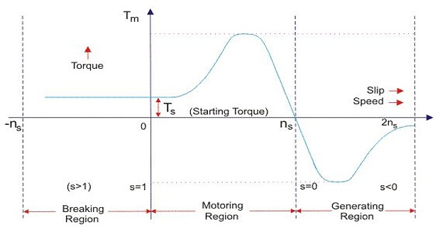
Low slip — the normal working region. The curve is a straight line through the origin.
Medium slip — the curve bends over and reaches its maximum at \(s_{max} = R_2/X_{20}\).
High slip — the torque falls away roughly as \(1/s\), reaching \(T_{st}\) at \(s = 1\).
At \(N_s\), \(s = 0\) and therefore the torque is zero — the starting point of the curve at the origin.
The Low-Slip Region
When \(N_r \approx N_s\), the slip \(s\) is very low and \(\left(sX_{20}\right)^{2}\) is negligible compared with \(R_2^{2}\). The torque equation therefore reduces to
As \(R_2\) is constant and \(E_{20}\) is fixed by the supply, the torque becomes
Hence, in the normal working region of the motor, the value of the slip is small and the torque-slip curve is a straight line.
The High-Slip Region
As the slip continues to rise, the term \(\left(sX_{20}\right)^{2}\) becomes large, and \(R_2^{2}\) may then be neglected in comparison with it. The torque becomes
The torque is inversely proportional to the slip. Beyond \(T_{max}\), the value of \(T\) starts decreasing — so a further increase in load, which raises the slip, actually reduces the torque available.
As a result the motor slows down and stops. At this stage the overload protection must immediately disconnect the motor from the supply, to prevent damage from overheating.
The machine does not simply settle at a lower speed; it collapses. Section 62-4 explains why the process is a runaway rather than a new equilibrium.
Problem. For the reference machine (\(E_{20} = 120\) V, \(R_2 = 0.25~\Omega\), \(X_{20} = 1.20~\Omega\), \(K_1 = 0.019099\)), compare the exact torque with each approximation across the slip range.
| \(s\) | Exact | \(K_1sE_{20}^{2}/R_2\) | Error | \(K_1E_{20}^{2}R_2/sX_{20}^{2}\) | Error |
|---|---|---|---|---|---|
| 0.01 | 10.976 | 11.001 | +0.23 % | 4775 | hopeless |
| 0.02 | 21.80 | 22.00 | +0.92 % | 2387 | hopeless |
| 0.04 | 42.44 | 44.00 | +3.69 % | 1194 | hopeless |
| 0.10 | 89.41 | 110.01 | +23.0 % | 477.5 | +434 % |
| 0.2083 | 114.59 | 229.18 | +100 % | 229.18 | +100 % |
| 0.50 | 81.37 | 550.0 | hopeless | 95.49 | +17.4 % |
| 1.00 | 45.76 | 1100 | hopeless | 47.75 | +4.34 % |
Working, the low-slip form at \(s = 0.04\).
Comment. The straight-line approximation is excellent below about \(s = 0.05\) — under 1 % error at 2 % slip, which covers the whole normal working range of most machines. The inverse-slip form is good above about \(s = 0.5\), reaching 4.3 % error at standstill.
Note the middle row. \(s_{max}\) is exactly where \(sX_{20} = R_2\), so neither term may be neglected — and both approximations give exactly twice the true value, since each drops one of two equal terms from the denominator. That coincidence marks the boundary between the two regimes precisely.
Stability and Pull-Out
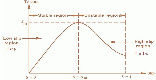
The motor operates between \(s = 0\) and \(s = s_{max}\). That restriction is not a convention but a consequence of stability.
Load rises → speed falls → slip rises → torque rises → balance restored at a slightly lower speed.
Self-correcting.
Load rises → speed falls → slip rises → torque falls further → speed falls further still.
A runaway. The motor stalls.
For a typical induction motor the pull-out torque is 2 to 3 times the rated full-load torque.
\(T_{st}\) is about 1.5 times the rated full-load torque.
The pull-out factor is a margin against stalling, not a usable rating. The machine can carry it only momentarily, because operating there means running at \(s_{max}\), where — by Chapter 63 — a fifth or more of the air-gap power is being dissipated in the rotor.
The reference machine has \(T_{max}/T_{fl} = 114.59/42.44 = 2.70\), comfortably within the usual band. A factor much below 2 would leave too little margin for load surges; much above 3 usually means the machine is larger than the duty requires.
Where the Load Line Cuts the Curve
A constant-torque load appears on the diagram as a horizontal line. Because the curve rises and then falls, that line generally cuts it twice — and the two intersections are of quite different character.
Problem. The reference machine drives a constant-torque load of 100 N m. Find both slips at which the developed torque equals the load, and identify which is the operating point.
Setting up. With \(K_1E_{20}^{2} = 275.02\):
Solving.
Identifying them. Since \(s_{max} = 0.20833\):
| \(s\) | Speed | Position | Character | |
|---|---|---|---|---|
| First | 0.12215 | 1316.8 rev/min | Below \(s_{max}\) | STABLE — the operating point |
| Second | 0.35531 | 967.0 rev/min | Above \(s_{max}\) | UNSTABLE — never settled at |
Comment. Both satisfy the equation exactly — substituting either back gives 100.00 N m. Mathematics alone cannot distinguish them; only the stability argument can.
Follow what happens on starting. The machine begins at \(s = 1\) with 45.76 N m — less than the 100 N m demanded, so it cannot start this load at all. Had the load been smaller, say 40 N m, the machine would accelerate from standstill, sweep leftwards past the peak, and settle at the low-slip intersection, never lingering at the high-slip one.
The 100 N m load is therefore startable only with rotor resistance added — which is exactly the case Section 62-9 examines.
Mode 1 · Motoring
The motor always rotates below the synchronous speed.
The slip varies from 0 at no load to 1 at standstill.
In the low-slip region the torque is directly proportional to the slip, and the linear relationship simplifies the calculation of motor performance to a great extent.
It is sometimes said that "the torque varies from zero to full-load torque as the slip varies from 0 to 1", and that the torque is proportional to slip over that whole range. Neither is quite right.
Table 62.1 shows the proportionality failing badly by \(s = 0.10\) — a 23 % error — and reversing altogether beyond \(s_{max}\). The torque does not increase monotonically to standstill; it peaks at \(s_{max}\) and then falls. In the reference machine it reaches 114.59 N m at \(s = 0.208\) and has fallen back to 45.76 N m by \(s = 1\).
Correctly stated: torque is proportional to slip in the low-slip working region only, and the full-load point lies within that region.
Mode 2 · Generating
The machine runs above the synchronous speed and must be driven by a prime mover.
Torque and slip are both negative.
It receives mechanical energy and delivers electrical energy — the stator winding now supplies energy to the mains instead of drawing it.
Nothing new is needed. The torque equation with \(s \lt 0\) gives a negative torque of the same magnitude as at the corresponding positive slip.
Running 60 rev/min above synchronous speed is electrically the mirror image of running 60 rev/min below it — the relative motion is the same size but in the opposite sense.
Older texts state that induction generators are not used, because they require reactive power for excitation which must be supplied from outside, and because if the speed falls below synchronous they consume electrical energy rather than delivering it.
Both facts are correct, but the conclusion no longer is. The induction generator is now the standard machine in wind turbines and small hydro schemes, precisely because it needs no excitation system, no synchronising equipment and no brush gear of its own — the grid supplies the reactive power, and the machine simply connects and delivers.
The genuine limitation is that it cannot run islanded without a capacitor bank or a converter to supply the magnetising current. Where a grid connection exists, that limitation costs nothing.
Mode 3 · Braking
Two leads, and hence the phase sequence, are interchanged so that the field reverses. The motor is driven to stop rapidly.
Used when the motor must stop within a very short period.
The kinetic energy stored in the revolving load is dissipated as heat, so the motor develops enormous heat energy.
For this reason the motor is disconnected from the supply the moment it reaches zero speed, or it would simply accelerate in reverse.
If the load driven by the motor accelerates it in the same direction as it is rotating — an overhauling load such as a descending hoist — the speed may rise above synchronous.
The motor then acts as an induction generator, supplying electrical energy to the mains.
That energy comes from the load, which is therefore slowed towards synchronous speed.
Energy is recovered, not wasted — the great advantage over plugging.
Problem. For the reference machine, tabulate slip, torque and rotor current at rotor speeds of \(-1440\), 0, 1200, 1440, 1500 and 1560 rev/min.
| \(N\) | \(s\) | \(T\) (N m) | \(I_2\) (A) | Mode |
|---|---|---|---|---|
| −1440 | 1.9600 | 24.09 | 99.44 | Braking (plugging) |
| 0 | 1.0000 | 45.76 | 97.90 | Standstill |
| 1200 | 0.2000 | 114.50 | 69.25 | Motoring, near peak |
| 1440 | 0.0400 | 42.44 | 18.86 | Motoring, full load |
| 1500 | 0.0000 | 0.00 | 0.00 | Synchronous |
| 1560 | −0.0400 | −42.44 | 18.86 | Generating |
Working, the plugging row.
Comment. The plugging row is the one to dwell on. The braking torque is only 24.09 N m — 21.0 % of \(T_{max}\) — yet the rotor current of 99.44 A is larger than the 97.90 A drawn at standstill.
Plugging is therefore a thermally brutal way to obtain a rather modest braking torque. The rotor is absorbing power from the supply and from the decelerating load simultaneously, and every watt of it becomes heat in the bars.
Compare the motoring and generating rows at \(s = \pm0.04\): identical magnitudes of torque and current, opposite signs of torque. The same equation covers the whole range from \(s = -0.04\) to \(s = 1.96\) without modification.
Effect of \(R_2\) on the Characteristic
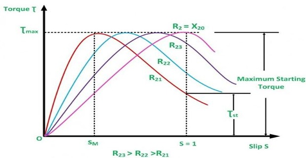
Chapter 61 proved that
\(T_{max}\) is independent of \(R_2\).
Therefore the effect of a change in \(R_2\) is a change in the slip at which \(T_{max}\) takes place.
The greater the \(R_2\), the greater the slip at which \(T_{max}\) occurs, since \(s_{max} = R_2/X_{20}\).
\(T_{max}\) can be obtained at the start by adding enough resistance in the rotor circuit that \(R_2 = X_{20}\).
When \(R_2 = X_{20}\), then \(s_{max} = R_2/X_{20} = 1\), that is \(T_{st} = T_{max}\).
Problem. For the reference machine, tabulate \(s_{max}\), \(T_{max}\) and \(T_{st}\) for rotor resistances of 0.25, 0.50, 0.80 and 1.20 Ω per phase.
| \(R_2\) (Ω) | \(s_{max}\) | \(T_{max}\) (N m) | \(T_{st}\) (N m) | \(T_{st}/T_{max}\) |
|---|---|---|---|---|
| 0.25 | 0.2083 | 114.59 | 45.76 | 39.93 % |
| 0.50 | 0.4167 | 114.59 | 81.37 | 71.01 % |
| 0.80 | 0.6667 | 114.59 | 105.78 | 92.31 % |
| 1.20 | 1.0000 | 114.59 | 114.59 | 100 % |
Working, the third row.
Comment. The third column is constant to five figures down the whole table. Adding rotor resistance buys starting torque without costing anything at the peak — the improvement from 45.76 to 114.59 N m is pure gain in the starting duty.
Return to the 100 N m load of Example 62.2, which the machine as built could not start. With \(R_2 = 0.80~\Omega\) the starting torque is 105.78 N m, comfortably above it, and the machine accelerates away. The rheostat is then cut out in steps as the speed rises, each step handing the machine over to a curve whose peak lies further to the left.
What the added resistance does cost is efficiency in the running condition. Chapter 63 shows that the rotor dissipates a fraction \(s\) of the air-gap power, so a machine deliberately run at high slip to control its speed is throwing away that same fraction as heat.
Problem. A 4-pole, 50 Hz motor has a full-load torque of 42.44 N m at 4 % slip and a pull-out factor of 2.70. A load requiring 60 N m is applied. Can the machine start it? Can it run it? What resistance would allow both?
Can it run it? The maximum torque is
Yes — 60 N m lies well below the peak, so a stable operating point exists on the rising part of the curve.
Can it start it? The starting torque is 45.76 N m.
The machine would sit at standstill drawing its full starting current, developing less torque than the load demands, and would overheat.
What resistance suffices? Require \(T_{st} \ge 60\):
Comment. Any rotor resistance between 0.339 and 4.244 Ω gives at least 60 N m at starting, so the external resistance may be anywhere from 0.089 to 3.994 Ω per phase.
The existence of an upper limit is the point worth noticing. Too much resistance is as useless as too little — beyond \(R_2 = X_{20}\) the peak has already passed \(s = 1\) and the starting torque falls again, exactly as Section 61-4 described.
In practice one would choose near \(R_2 = X_{20} = 1.20~\Omega\) to obtain the full 114.59 N m, giving a healthy margin for acceleration rather than the bare minimum.
Summary and Key Formulas
The curve has three regions: low slip (a straight line), medium slip (bending to the peak at \(s_{max}\)), and high slip (falling as \(1/s\)).
Low slip: \((sX_{20})^{2} \ll R_2^{2}\) so \(T \approx K_1sE_{20}^{2}/R_2\) and \(T \propto s\). Under 1 % error at 2 % slip.
High slip: \(R_2^{2}\) negligible, so \(T \approx K_1E_{20}^{2}R_2/sX_{20}^{2}\) and \(T \propto 1/s\). About 4 % error at standstill.
At \(s_{max}\) the two terms are equal, so both approximations give exactly twice the true value.
Only \(0 \lt s \lt s_{max}\) is stable. Beyond the peak, more load means less torque, and the machine stalls rather than settling.
A constant-torque load line cuts the curve twice; only the low-slip intersection is a real operating point.
Typical design figures: pull-out 2 to 3 × full-load torque, \(T_{st}\) about 1.5 × full-load torque.
Motoring \(0 \lt s \lt 1\); generating \(s \lt 0\), torque and slip both negative; braking \(s \gt 1\).
Plugging reverses the phase sequence: fast stop, enormous rotor heat, and the supply must be removed at zero speed. Regenerative braking occurs on an overhauling load and returns energy to the mains.
\(T_{max}\) is independent of \(R_2\). Raising \(R_2\) moves the peak to higher slip; \(R_2 = X_{20}\) puts it at \(s = 1\), so \(T_{st} = T_{max}\).
| Quantity | Formula | Notes |
|---|---|---|
| Torque | \(T = \dfrac{K_1sE_{20}^{2}R_2}{R_2^{2}+\left(sX_{20}\right)^{2}}\) | covers every mode |
| Low-slip form | \(T \approx \dfrac{K_1sE_{20}^{2}}{R_2}\) | \(T\propto s\), good to \(s\approx0.05\) |
| High-slip form | \(T \approx \dfrac{K_1E_{20}^{2}R_2}{sX_{20}^{2}}\) | \(T\propto 1/s\), good above \(s\approx0.5\) |
| Slip at peak | \(s_{max} = \dfrac{R_2}{X_{20}}\) | where \(sX_{20}=R_2\) |
| Peak torque | \(T_{max} = \dfrac{K_1E_{20}^{2}}{2X_{20}}\) | no \(R_2\) |
| Stable region | \(0 \lt s \lt s_{max}\) | — |
| Pull-out factor | \(T_{max}/T_{fl}\) | 2 to 3 typically |
| Max torque at start | \(R_2 = X_{20}\) | gives \(s_{max}=1\) |
| Mode from slip | \(s\lt0\), \(0\lt s\lt1\), \(s\gt1\) | generator, motor, brake |
Common Mistakes
Saying torque is proportional to slip over the whole range. It holds only at low slip; beyond \(s_{max}\) the torque falls as slip rises.
Believing the torque is greatest at standstill. The peak is at \(s_{max} = R_2/X_{20}\), typically 0.15 to 0.3 for a cage machine.
Treating the high-slip intersection as an operating point. It is unstable and never settled at.
Thinking pull-out torque is a continuous rating. It is a momentary margin — the rotor loss at \(s_{max}\) is enormous.
Expecting \(T_{max}\) to rise with rotor resistance. It never changes; only \(s_{max}\) moves.
Assuming more rotor resistance always helps starting. Beyond \(R_2 = X_{20}\) the starting torque falls again.
Leaving the plugging supply connected past zero speed. The machine accelerates in reverse.
Confusing plugging with regenerative braking. Plugging wastes energy as rotor heat; regenerative braking returns it to the supply.
Dismissing the induction generator. It is the standard wind-turbine machine; it simply cannot run islanded without capacitors.
Assuming large braking torque during plugging. In Example 62.3 it is only 21 % of \(T_{max}\), for more current than at standstill.
Chapter Review
Throughout, \(K_1E_{20}^{2} = 275.02\) for the reference machine, so \(T = 275.02\,sR_2/[R_2^{2}+1.44s^{2}]\).
P62.1 A motor has \(R_2 = 0.30~\Omega\) and \(X_{20} = 1.00~\Omega\). Find \(s_{max}\) and the speed at which peak torque occurs, given \(N_s = 1000\) rev/min.
Show answer
\[s_{max} = \frac{0.30}{1.00} = 0.300\]\[N = (1-0.300)(1000) = 700~\mathrm{rev/min}\]P62.2 For the reference machine, find the torque at \(s = 0.02\) both exactly and by the low-slip approximation, and give the error.
Show answer
\[T_{exact} = \frac{(275.02)(0.02)(0.25)}{0.0625+(1.44)(0.0004)} = \frac{1.3751}{0.063076} = 21.80~\mathrm{N\,m}\]\[T_{approx} = \frac{(275.02)(0.02)}{0.25} = 22.00~\mathrm{N\,m}\]\[\text{error} = \frac{22.00-21.80}{21.80}\times100 = +0.92\,\%\]P62.3 A machine has \(T_{fl} = 50\) N m at 4 % slip and a pull-out factor of 2.5. Find \(T_{max}\), and state whether a 120 N m load can be carried.
Show answer
Since \(120 \lt 125\), the load can be carried — but with only 4 % margin, so any surge or voltage dip would stall the machine.\[T_{max} = (2.5)(50) = 125~\mathrm{N\,m}\]P62.4 The reference machine drives a 60 N m constant-torque load. Find the operating slip and speed.
Show answer
\[\frac{68.755\,s}{0.0625+1.44s^{2}} = 60 \quad\Longrightarrow\quad 86.40s^{2} - 68.755s + 3.750 = 0\]\[\Delta = 4727.24 - 1296.0 = 3431.24, \qquad \sqrt{\Delta} = 58.577\]The operating point is the stable one, \(s_1 = 0.0589\):\[s = \frac{68.755 \pm 58.577}{172.80} \quad\Longrightarrow\quad s_1 = 0.05890,\ s_2 = 0.73688\]\[N = (1-0.0589)(1500) = 1411.6~\mathrm{rev/min}\]P62.5 A 4-pole 50 Hz machine runs at 1560 rev/min driven by a turbine. Find the slip and state the mode.
Show answer
Negative slip: the machine is generating, delivering electrical energy to the supply while absorbing mechanical energy from the turbine. Torque and slip are both negative.\[s = \frac{1500-1560}{1500} = -0.0400\]P62.6 For the reference machine, what rotor resistance places \(T_{max}\) at a slip of 0.60, and what is \(T_{st}\) then?
Show answer
\[R_2 = s_{max}X_{20} = (0.60)(1.20) = 0.72~\Omega \quad\Longrightarrow\quad R_{ext} = 0.47~\Omega\]\[T_{st} = \frac{(275.02)(0.72)}{(0.72)^{2}+1.44} = \frac{198.01}{1.9584} = 101.11~\mathrm{N\,m}\]P62.7 Explain why only the region between \(s = 0\) and \(s_{max}\) is stable.
Show answer
Consider a small increase in load torque and follow the consequences.Left of the peak (\(s \lt s_{max}\)): the rotor slows, so the slip rises, and on this part of the curve a higher slip means a higher torque. The developed torque therefore rises to meet the new load, and the machine settles at a slightly lower speed. Self-correcting.
Right of the peak (\(s \gt s_{max}\)): the rotor slows, the slip rises, but here a higher slip means a lower torque. The shortfall grows, the machine slows further, the torque falls further still. A runaway.
The motor therefore decelerates all the way to standstill — it stalls. The overload protection must disconnect it immediately, since it will otherwise sit drawing locked-rotor current and overheat within seconds.
The mathematical statement: stability requires \(dT/ds \gt 0\), which holds precisely for \(s \lt s_{max}\).
P62.8 A constant-torque load line cuts the curve twice. Why is only one intersection a real operating point?
Show answer
Both intersections satisfy \(T_{developed} = T_{load}\) exactly, so both are equilibria in the mathematical sense. Only the stability argument distinguishes them.The low-slip intersection lies where \(dT/ds \gt 0\) and is stable, as P62.7 shows.
The high-slip intersection lies beyond the peak where \(dT/ds \lt 0\). Any disturbance is amplified: a slight slowing reduces the torque, which slows it further, and the machine runs away to standstill; a slight speeding-up increases the torque, and it accelerates away towards the low-slip point.
What actually happens on starting. The machine begins at \(s = 1\) with an excess of torque over the load, accelerates leftwards, passes through the unstable intersection without pausing, sweeps over the peak, and settles at the low-slip intersection.
In Example 62.2 those were \(s = 0.355\) (passed through) and \(s = 0.122\) (settled at).
P62.9 Compare plugging with regenerative braking.
Show answer
Plugging (\(s \gt 1\)). Two supply leads are interchanged, reversing the phase sequence and hence the field, while inertia keeps the rotor turning the old way. The relative motion becomes the sum of the two speeds.Torque reverses and brakes the machine rapidly — used when a very short stopping time is required.
The rotor absorbs power from the supply and the load's kinetic energy, and all of it becomes heat in the rotor.
The supply must be removed at zero speed, or the machine accelerates in reverse.
Thermally brutal for a modest torque: Example 62.3 gives 24.09 N m — 21 % of \(T_{max}\) — for 99.4 A, more current than at standstill.
The machine becomes an induction generator and delivers energy to the mains.
That energy comes from the load, which is therefore held back towards synchronous speed.
Energy is recovered rather than wasted, and the machine can hold a load at a steady speed indefinitely — which plugging cannot.
The choice: plugging when stopping time matters more than energy; regenerative braking whenever the load naturally overhauls.
P62.10 Explain the effect of rotor resistance on the family of torque-slip curves, and why it is useful.
Show answer
From Chapter 61,\(T_{max}\) contains no \(R_2\), but \(s_{max}\) is proportional to it. So raising the rotor resistance slides the peak to the right without changing its height.\[s_{max} = \frac{R_2}{X_{20}}, \qquad T_{max} = \frac{K_1E_{20}^{2}}{2X_{20}}\]Setting \(R_2 = X_{20}\) gives \(s_{max} = 1\), so the full maximum torque is available at the instant of starting: \(T_{st} = T_{max}\).
Why it is useful. Example 62.4 shows the starting torque rising from 45.76 to 114.59 N m — a 2.5-fold gain — at no cost to the peak. This is what allows a slip-ring motor to start a crane, hoist or crusher under full load.
The cost. Nothing at starting, but a great deal in running. Chapter 63 shows the rotor dissipates a fraction \(s\) of the air-gap power, so a machine held at high slip to control its speed wastes that same fraction as heat. The resistance is therefore cut out in steps as the machine accelerates, each step handing it to a curve whose peak lies further left.
MCQ 1. In the low-slip region the torque is proportional to:
(a) \(1/s\) (b) \(s\) (c) \(s^{2}\) (d) constantShow answer
(b) \(s\).MCQ 2. In the high-slip region the torque is proportional to:
(a) \(s\) (b) \(1/s\) (c) \(s^{2}\) (d) \(\sqrt{s}\)Show answer
(b) \(1/s\).MCQ 3. The stable operating region is:
(a) \(0 \lt s \lt s_{max}\) (b) \(s_{max} \lt s \lt 1\) (c) all of \(0 \lt s \lt 1\) (d) \(s \gt 1\)Show answer
(a) \(0 \lt s \lt s_{max}\), where \(dT/ds \gt 0\).MCQ 4. The pull-out torque of a typical machine is:
(a) 1.0 to 1.2 × \(T_{fl}\) (b) 2 to 3 × \(T_{fl}\) (c) 6 × \(T_{fl}\) (d) 10 × \(T_{fl}\)Show answer
(b) 2 to 3 × \(T_{fl}\).MCQ 5. Raising the rotor resistance changes:
(a) \(T_{max}\) only (b) \(s_{max}\) only (c) both (d) neitherShow answer
(b) \(s_{max}\) only — the peak slides but does not change height.MCQ 6. When \(R_2 = X_{20}\):
(a) \(T_{st} = 0\) (b) \(T_{st} = T_{max}\) (c) \(s_{max} = 0\) (d) the motor cannot startShow answer
(b) \(T_{st} = T_{max}\), since \(s_{max} = 1\).MCQ 7. During plugging the machine:
(a) generates (b) brakes with \(s \gt 1\) (c) runs at \(s = 0\) (d) motors normallyShow answer
(b) brakes with \(s \gt 1\), dissipating all the energy as rotor heat.MCQ 8. Regenerative braking occurs when:
(a) \(s \gt 1\) (b) \(s = 1\) (c) \(s \lt 0\) (d) \(s = s_{max}\)Show answer
(c) \(s \lt 0\) — the load drives the rotor above synchronous speed.MCQ 9. A horizontal load line generally cuts the torque-slip curve:
(a) once (b) twice (c) three times (d) neverShow answer
(b) twice, but only the low-slip intersection is stable.MCQ 10. At \(s = s_{max}\) both limiting approximations give:
(a) the exact value (b) half the true value (c) twice the true value (d) zeroShow answer
(c) twice the true value — each drops one of two equal denominator terms.
Sketch the torque-slip curve and identify its three regions.
Derive the low-slip and high-slip approximations and state where each is valid.
Explain why only the region below \(s_{max}\) is stable.
Explain why a load line cuts the curve twice and which intersection is real.
Describe the motoring, generating and braking modes in terms of slip.
Compare plugging with regenerative braking.
Explain the effect of rotor resistance on the family of curves.
What is the pull-out factor, and why is it a margin rather than a rating?
Two debts have now accumulated. Both are settled in Chapter 63, which follows the power stages from the stator terminals to the shaft.
The first is the claim, verified numerically in Example 61.4 but never proved, that the air-gap power divides in the ratio \(s : (1-s)\):
The second is the repeated assertion that operating at high slip is wasteful. The division above makes it exact and rather startling: a machine running at \(s_{max} = 0.208\) to obtain its peak torque is dissipating 20.8 % of everything crossing the air gap in the rotor bars, and one held at 50 % slip by rotor resistance is wasting half. That is why speed control by rotor resistance, for all its simplicity, has given way to the variable-frequency drive.
Chapter 63 also gives the ceiling on efficiency, \(\eta \le 1 - s\), before stator and mechanical losses are even counted — which is the cleanest possible statement of why an induction motor must run at low slip to be worth using at all.