By the end of this chapter you should be able to:
State the assumptions defining an ideal transformer.
Explain the role of the magnetising current and its phase relative to the applied voltage.
Derive the EMF equation \(E = 4.44fN\Phi_m\) from the average rate of change of flux.
Explain why the volts per turn is the same for both windings.
Define the transformation ratio and relate voltage, current and turns.
Apply the ampere-turn balance to find the currents.
Refer an impedance from one winding to the other.
Explain why the flux is fixed by the supply and not by the load.
The Ideal Transformer

An ideal transformer is one which has no losses: its windings have no ohmic resistance, there is no magnetic leakage, and hence there are no \(I^{2}R\) losses and no core losses.
In other words, it consists of two purely inductive coils wound on a loss-free core.
It is impossible to realise such a transformer in practice.
Because every real transformer is close to it. A large power transformer is 99.5 % efficient, its leakage flux is a few percent of the main flux, and its magnetising current is 1 to 3 % of full-load current. The ideal transformer is not a crude approximation but an excellent one, and every result derived here survives into the real machine with only small corrections.
Those corrections are the business of the next three chapters, each of which relaxes one assumption: Chapter 42 restores the magnetising current and core loss, Chapter 43 the winding resistance and leakage reactance, and Chapter 44 assembles them into the full equivalent circuit.
| Assumption | Removes | Restored in |
|---|---|---|
| No winding resistance | Copper loss, resistive volt drop | Chapter 43 |
| No leakage flux | Leakage reactance | Chapter 43 |
| Loss-free core | Hysteresis and eddy-current loss | Chapter 42 |
| Infinite core permeability | Magnetising current | Chapter 42 |
What Happens on No Load
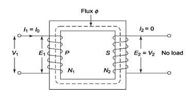
Consider an ideal transformer whose secondary is open and whose primary is connected to a sinusoidal alternating voltage \(V_1\).
- The potential difference causes an alternating current to flow in the primary.
- Since the primary coil is purely inductive and the secondary is open — no output — the primary draws a magnetising current \(I_\mu\) only.
- \(I_\mu\) is very small in magnitude, magnetises the core, and lags \(V_1\) by 90°.
- The alternating current \(I_\mu\) produces an alternating flux \(\Phi\), which at all times is proportional to the current and in phase with it.
This changing flux is linked with both \(N_1\) and \(N_2\), and therefore induces an EMF in each:
A self-induced EMF in the primary, \(E_1\), which at every instant opposes \(V_1\) — the counter EMF or back EMF of the primary.
A mutually induced EMF in the secondary, \(E_2\), in antiphase with \(V_1\).
The magnitude of \(E_2\) is proportional to the rate of change of flux and to the number of secondary turns.
The EMF Equation

Let
The flux increases from zero to its maximum value \(\Phi_m\) in one quarter of a cycle, that is in \(1/4f\) seconds. Therefore the average rate of change of flux is
Rate of change of flux per turn means induced EMF in volts, so
If the flux varies sinusoidally, the RMS value is obtained by multiplying the average by the form factor:
Multiplying by the number of turns in each winding gives the two EMFs:
The number is not arbitrary and not a fudge factor. It is \(4 \times 1.11\), and each factor has a distinct origin:
The 4 comes from the geometry of a quarter cycle — the flux swings through \(\Phi_m\) in \(1/4f\) seconds.
The 1.11 is the form factor of a sine wave, \(\pi/2\sqrt 2 = 1.1107\), converting average to RMS.
Change the waveform and 4.44 changes with it. For a square wave the form factor is 1, and the EMF equation becomes \(E = 4fN\Phi_m\) — which is why switched-mode transformers running on square waves handle more power from the same core.
Problem. A 50 Hz single-phase transformer has 200 primary and 50 secondary turns. The net core area is 0.008 m² and the maximum flux density 1.2 T. Find the flux, the volts per turn, and both EMFs.
Maximum flux.
Volts per turn.
The two EMFs.
Check via the ratio.
Comment. This is a step-down transformer, since \(N_2 \lt N_1\). Note that the flux never entered the ratio — it cancels, because both windings link the same flux. That cancellation is the whole reason a transformer's ratio depends only on turns.
Volts per Turn
Both windings are threaded by the same core flux and see the same frequency, so each turn — wherever it sits — has the same voltage induced in it. The windings differ only in how many such turns they contain.
This single fact is what makes transformer design tractable. The designer fixes \(E_t\) from the core — as Example 40.3 did — and every winding on that core then follows by simple division.
Problem. A 2200/220 V, 50 Hz transformer is to be built on a core of net area 0.02 m² working at 1.1 T. Find the volts per turn and the turns on each winding. Adjust to whole turns and state the resulting flux density.
Volts per turn.
Turns required.
Rounding. Take \(N_1 = 450\) and \(N_2 = 45\), which preserves the ratio exactly:
Resulting flux density.
Comment. Rounding down to 450 turns raises the volts per turn slightly, so the flux density rises from 1.100 to 1.101 T — a change of one part in a thousand, entirely acceptable.
The ratio 450 : 45 is exactly 10 : 1, so the secondary voltage lands precisely on 220 V. This is luck rather than design; when the numbers do not divide neatly, the designer adjusts the core area or the flux density until they do — which is why quoted flux densities are rarely round numbers.
The Transformation Ratio
Dividing the two EMF equations, the common factor \(4.44f\Phi_m\) cancels:
\(K\) is the transformation ratio, sometimes called the turns ratio. In an ideal transformer \(V_1 = E_1\) and \(V_2 = E_2\), so the voltage ratio and the EMF ratio are the same.
\(K \gt 1\) — step-up transformer.
\(K \lt 1\) — step-down transformer.
\(K = 1\) — isolating transformer, which changes nothing but the electrical connection.
For an ideal transformer, input VA equals output VA, since there are no losses:
Current and Ampere-Turn Balance
Combining \(I_2/I_1 = 1/K\) with \(K = N_2/N_1\) gives an equivalent and often more useful statement:
The flux is set by \(V_1\) and cannot alter while the supply is fixed. So when the secondary carries \(I_2\), its MMF \(N_2I_2\) would tend to change the flux — and the primary must immediately draw a further current \(I_1\) whose MMF \(N_1I_1\) exactly cancels it.
The secondary MMF is neutralised as fast as it appears, leaving only the small magnetising MMF to maintain the flux.
This is the transformer's version of the self-regulation seen in Chapter 34. The primary does not "know" the load; it responds automatically because any imbalance in ampere-turns would disturb the flux, and disturbing the flux immediately alters \(E_1\), which changes the primary current until balance is restored.
Problem. The transformer of Example 41.2 (2200/220 V, 450/45 turns) is rated at 50 kVA. Find the full-load currents on both sides and verify the ampere-turn balance.
Currents.
Ratio check.
Ampere-turn balance.
Comment. The currents are in the inverse ratio of the turns, so the ampere-turns match exactly. This gives a quick sanity check on any transformer calculation: if \(N_1I_1 \ne N_2I_2\), something is wrong.
Note the practical consequence for construction. The secondary carries ten times the current in a tenth of the turns, so its conductor must have roughly ten times the cross-section. The two windings occupy similar volumes of copper — which is why the window of a transformer is divided roughly equally between them, whatever the ratio.
Referring Impedance
Because the transformer scales voltage by \(K\) and current by \(1/K\), it scales impedance by the square of the ratio. This is the most useful single idea in transformer analysis.
A load \(Z_2\) on the secondary draws \(I_2 = V_2/Z_2\). Seen from the primary terminals:
So to refer a quantity from secondary to primary:
Referring changes the numbers but not the power, since \(I'^{2}Z' = (KI)^{2}(Z/K^{2}) = I^{2}Z\).
The consequence is that a transformer with a load can be replaced by a single impedance on the primary side, and the whole two-circuit problem collapses to one circuit. Chapter 44 uses this to fold the secondary resistance and leakage reactance into the primary, producing the equivalent circuit that carries the rest of Part 3.
Because \(K\) can be chosen freely, a transformer can make any load look like any impedance. This is used for maximum power transfer — Chapter 4's theorem — where the source resistance must be matched.
An 8 \(\Omega\) loudspeaker driven from an amplifier needing a 3200 \(\Omega\) load requires \(K^{2} = 8/3200\), that is \(K = 1/20\). The transformer is acting purely as an impedance converter, not to change the voltage for its own sake.
Problem. A 4 \(\Omega\) resistive load is connected to the 220 V secondary of the 2200/220 V transformer of Example 41.2. Find the impedance seen at the primary terminals, the two currents, and verify that the power is the same computed either way.
Referred impedance. Here \(K = 220/2200 = 0.1\):
Currents.
Check from the primary side.
Power both ways.
Comment. The 4 \(\Omega\) load appears as 400 \(\Omega\) — a hundredfold increase, because \(K^{2} = 1/100\). The current is a tenth and the impedance a hundred times, but the power is identical, which is the consistency check to apply whenever referring.
A useful habit: once referred, forget the transformer exists. The primary circuit is now simply 2200 V across 400 \(\Omega\), and every ordinary circuit technique applies unchanged.
The Flux Is Fixed by the Supply
Rearranging the EMF equation exposes a fact that governs transformer behaviour everywhere in Part 3.
With \(V_1\), \(f\) and \(N_1\) all fixed, \(\Phi_m\) is fixed. The load current does not appear.
Two consequences follow immediately:
The iron loss is constant at all loads, since it depends on \(B_m\) and \(f\) — which is exactly the assumption Chapter 46 relies on when it measures iron loss by an open-circuit test at no load.
The magnetising current is constant at all loads.
Contrast the DC machine of Part 2, where armature reaction let the load current distort and weaken the field. A transformer has no such effect, because the ampere-turn balance cancels the secondary MMF.
The same expression shows what happens if the supply changes. Since \(B_m \propto V_1/f\), it is the volts per hertz that matters, not the voltage alone — a rule that recurs throughout AC machine practice.
Problem. A transformer is designed for 220 V, 50 Hz with \(B_m = 1.1\) T. Find the flux density if it is operated at 220 V but (a) 60 Hz and (b) 25 Hz. Comment on each, and state how the iron losses scale.
The governing relation.
(a) At 60 Hz.
Perfectly safe. The core is simply under-used, and the machine could carry a higher voltage at this frequency.
(b) At 25 Hz.
Above the saturation value of about 2 T from Chapter 40. The core saturates, the magnetising current rises enormously, and the transformer will overheat and may burn out.
How the iron losses scale at constant voltage. Using \(P_h \propto fB_m^{1.6}\) and \(P_e \propto f^{2}B_m^{2}\) with \(B_m \propto 1/f\):
| Frequency | \(B_m\) | Hysteresis | Eddy current |
|---|---|---|---|
| 60 Hz | 0.917 T | 0.896 | 1.000 |
| 50 Hz | 1.100 T | 1.000 | 1.000 |
| 25 Hz | 2.200 T | 1.516 | 1.000 |
Comment. The eddy-current column is exactly 1.000 at every frequency, and this is no coincidence:
At constant applied voltage the eddy-current loss depends only on the voltage, not on the frequency at all. The hysteresis loss does vary, falling at higher frequency because the reduced flux density more than compensates the extra cycles.
The practical rule: a transformer may safely be used at a higher frequency than its rating, but never at a lower one unless the voltage is reduced in proportion. A 50 Hz unit on 60 Hz is fine; a 60 Hz unit on 50 Hz is running 20 % over-fluxed.
Polarity and the Dot Convention
The EMF equation gives magnitudes. The relative sense of the two windings is shown by dots marked on the terminals.
Terminals marked with a dot are those which, at any instant, have the same instantaneous polarity.
Equivalently: current entering the dotted terminal of one winding produces flux in the same direction as current entering the dotted terminal of the other.
For a single transformer feeding an isolated load, the polarity is irrelevant. It becomes essential for
parallel operation, where opposing polarities cause a short circuit;
autotransformer connections;
three-phase banks, where the group and phase displacement depend on it.
Two conventions are used in practice: additive polarity, where the induced voltages add around the loop when adjacent terminals are joined, and subtractive polarity, where they oppose. Subtractive polarity is standard for large transformers, because it keeps the voltage between adjacent bushings low.
Summary and Key Formulas
An ideal transformer has no winding resistance, no leakage flux, no core loss and infinite permeability. It cannot be realised, but a real transformer is close to it.
On no load the primary draws only the magnetising current \(I_\mu\), which lags \(V_1\) by 90° and is in phase with the flux it produces.
The flux covers \(\Phi_m\) in a quarter cycle, giving an average EMF per turn of \(4f\Phi_m\); multiplying by the form factor 1.11 gives \(4.44f\Phi_m\).
Volts per turn is the same on both windings, because both link the same flux at the same frequency.
The transformation ratio is \(K = N_2/N_1 = E_2/E_1 = V_2/V_1\), and \(I_2/I_1 = 1/K\).
Ampere-turns balance: \(N_1I_1 = N_2I_2\). The secondary MMF is cancelled as fast as it appears, so the flux is undisturbed.
Impedance refers as \(K^{2}\): \(Z' = Z/K^{2}\), with \(V' = V/K\) and \(I' = KI\). Power is unchanged.
Flux is fixed by the supply, \(\Phi_m = V_1/4.44fN_1\), so iron loss and magnetising current are constant at all loads. What matters is the volts per hertz.
| Quantity | Formula | Notes |
|---|---|---|
| Maximum flux | \(\Phi_m = B_mA\) | \(A\) is net iron area |
| Average EMF per turn | \(4f\Phi_m\) | quarter-cycle argument |
| Form factor | \(\pi/2\sqrt2 = 1.11\) | sine wave only |
| EMF per turn (RMS) | \(E_t = 4.44f\Phi_m\) | same both windings |
| EMF equation | \(E_1 = 4.44fN_1\Phi_m\) | likewise \(E_2\) with \(N_2\) |
| Transformation ratio | \(K = \dfrac{N_2}{N_1} = \dfrac{E_2}{E_1} = \dfrac{V_2}{V_1}\) | step-up if \(K \gt 1\) |
| Current ratio | \(\dfrac{I_2}{I_1} = \dfrac{1}{K}\) | from \(V_1I_1 = V_2I_2\) |
| Ampere-turn balance | \(N_1I_1 = N_2I_2\) | useful check |
| Referred impedance | \(Z' = Z/K^{2}\) | secondary to primary |
| Flux from supply | \(\Phi_m = \dfrac{V_1}{4.44fN_1}\) | \(B_m \propto V_1/f\) |
| Eddy loss at constant \(V\) | \(P_e \propto V_1^{2}\) | independent of \(f\) |
Common Mistakes
Writing 4.44 as 4. The 4 is the quarter-cycle factor; the form factor 1.11 must multiply it.
Using peak instead of RMS. \(4.44fN\Phi_m\) gives the RMS EMF directly.
Using \(B_m\) with the gross core area. Use the net iron area, \(k_sA_{\text{gross}}\).
Defining \(K\) upside down. Here \(K = N_2/N_1\), so \(K \gt 1\) means step-up. Some books use the reciprocal — check before quoting a formula.
Referring impedance with \(K\) instead of \(K^{2}\). Voltage and current each scale by \(K\), so impedance scales by its square.
Thinking the flux depends on the load. It is set by \(V_1\), \(f\) and \(N_1\) alone.
Expecting the frequency to change. Both sides are always at supply frequency.
Running a transformer at reduced frequency at rated voltage. \(B_m \propto V/f\), so the core saturates.
Forgetting the power check after referring. \(I'^{2}Z'\) must equal \(I^{2}Z\).
Ignoring polarity when paralleling. Opposed polarities produce a short circuit.
Chapter Review
Find the volts per turn first; almost everything else follows by multiplication or division.
P41.1 A 50 Hz transformer has a net core area of 0.012 m² and works at 1.5 T. Find the volts per turn.
Show answer
\[\Phi_m = (1.5)(0.012) = 0.0180~\mathrm{Wb}\]\[E_t = (4.44)(50)(0.0180) = 3.996~\mathrm{V/turn}\]P41.2 For P41.1, find the turns for a 3300/240 V transformer.
Show answer
With 826 and 60 turns, \(K = 60/826 = 0.07264\) and the actual secondary voltage is \((0.07264)(3300) = 239.7\) V.\[N_1 = \frac{3300}{3.996} = 825.8 \to 826, \qquad N_2 = \frac{240}{3.996} = 60.1 \to 60\]P41.3 A 400/100 V transformer supplies 20 A to its secondary. Find \(K\), the primary current and the ampere-turns if \(N_2 = 50\).
Show answer
\[K = \frac{100}{400} = 0.25, \qquad I_1 = KI_2 = (0.25)(20) = 5~\mathrm{A}\]\[N_1 = \frac{50}{0.25} = 200, \qquad N_1I_1 = 1000 = N_2I_2 = (50)(20) \quad\checkmark\]P41.4 A 25 \(\Omega\) load is on the secondary of a 1100/220 V transformer. Find the referred impedance and both currents.
Show answer
\[K = 0.2, \qquad Z' = \frac{25}{0.04} = 625~\Omega\]\[I_2 = \frac{220}{25} = 8.8~\mathrm{A}, \qquad I_1 = (0.2)(8.8) = 1.76~\mathrm{A}\]\[\text{check: } \frac{1100}{1.76} = 625~\Omega \quad\checkmark\]P41.5 An amplifier requires a 4500 \(\Omega\) load and drives a 5 \(\Omega\) loudspeaker. Find the turns ratio needed.
Show answer
A 30 : 1 step-down transformer. For 900 primary turns, the secondary would have 30.\[K^{2} = \frac{Z_2}{Z'} = \frac{5}{4500} = \frac{1}{900} \quad\Longrightarrow\quad K = \frac{1}{30}\]P41.6 A transformer designed for 400 V, 50 Hz is connected to 400 V, 40 Hz. Find the change in flux density and comment.
Show answer
The flux density rises 25 %. If the design value was 1.5 T it becomes 1.875 T, approaching saturation — the magnetising current would rise sharply and the transformer would overheat. To use it at 40 Hz the voltage must be reduced to \((400)(40/50) = 320\) V.\[\frac{B_2}{B_1} = \frac{f_1}{f_2} = \frac{50}{40} = 1.25\]P41.7 Derive the EMF equation, stating the origin of each factor in 4.44.
Show answer
The flux rises from zero to \(\Phi_m\) in a quarter cycle, that is in \(1/4f\) seconds, so the average rate of change is \(\Phi_m/(1/4f) = 4f\Phi_m\) Wb/s. Rate of change of flux per turn is EMF in volts, so the average EMF per turn is \(4f\Phi_m\).For a sinusoid the RMS value is the average multiplied by the form factor \(\pi/2\sqrt2 = 1.11\), giving \(E_t = 4.44f\Phi_m\) and hence \(E = 4.44fN\Phi_m\).
Origins: the 4 is geometric — the flux traverses its full amplitude in a quarter period. The 1.11 is the sine wave's form factor. A square-wave supply would give 4.00, not 4.44.
P41.8 Explain why the volts per turn is the same for both windings.
Show answer
Both windings are wound on the same core and are therefore linked by the same flux, alternating at the same frequency. Faraday's law says the EMF induced in a single turn is the rate of change of the flux linking it — so every turn on that core, in whichever winding, has the same EMF induced in it.The windings differ only in how many such turns they contain, which is why \(E_1/N_1 = E_2/N_2 = 4.44f\Phi_m\).
This is why leakage flux matters: it is precisely the flux that links one winding but not the other, and it is the reason a real transformer's volts per turn differ slightly between windings.
P41.9 Explain why the core flux is independent of the load, and give two consequences.
Show answer
From the EMF equation, \(\Phi_m = V_1/(4.44fN_1)\) — and no load current appears. With the supply voltage, frequency and primary turns all fixed, the flux is fixed.Mechanism: when the secondary carries current, its MMF \(N_2I_2\) would tend to alter the flux. Any such change alters \(E_1\), which unbalances \(V_1 - E_1\) and immediately draws additional primary current until \(N_1I_1 = N_2I_2\). The secondary MMF is cancelled as fast as it appears.
Consequences: the iron loss is constant at all loads (so it can be measured at no load, as Chapter 46 does), and the magnetising current is constant at all loads.
P41.10 Why may a 50 Hz transformer be used on 60 Hz but not the reverse?
Show answer
Because \(B_m \propto V_1/f\). At higher frequency and the same voltage the flux density falls, so a 50 Hz unit on 60 Hz works at \(50/60 = 83\) % of its design flux density — safe, merely under-using the core.At lower frequency the flux density rises. A 60 Hz unit on 50 Hz runs at \(60/50 = 120\) % of design flux density, and since the design point is already near the knee of the B-H curve, the core saturates. The magnetising current rises steeply and non-sinusoidally, and the transformer overheats.
The remedy is to reduce the voltage in proportion, keeping the volts per hertz at its design value.
MCQ 1. An ideal transformer has:
(a) no losses and no leakage (b) small losses (c) unity ratio (d) an air coreShow answer
(a) no losses and no leakage, and infinite core permeability.MCQ 2. On no load the magnetising current lags the applied voltage by:
(a) 0° (b) 45° (c) 90° (d) 180°Show answer
(c) 90°, the primary being purely inductive in the ideal case.MCQ 3. The factor 4.44 is the product of:
(a) 2 and 2.22 (b) 4 and 1.11 (c) π and 1.41 (d) 4.44 and 1Show answer
(b) 4 and 1.11 — the quarter-cycle factor and the form factor.MCQ 4. The EMF per turn in a transformer is:
(a) larger on the primary (b) larger on the secondary (c) the same on both (d) zeroShow answer
(c) the same on both, since both link the same flux at the same frequency.MCQ 5. If \(K = N_2/N_1 \gt 1\), the transformer is:
(a) step-down (b) step-up (c) isolating (d) impossibleShow answer
(b) step-up. More secondary turns give a higher secondary voltage.MCQ 6. In an ideal transformer the currents are related by:
(a) \(I_2/I_1 = K\) (b) \(I_2/I_1 = 1/K\) (c) \(I_2 = I_1\) (d) \(I_2/I_1 = K^{2}\)Show answer
(b) \(I_2/I_1 = 1/K\) — current transforms inversely to voltage.MCQ 7. An impedance \(Z\) on the secondary appears on the primary as:
(a) \(KZ\) (b) \(Z/K\) (c) \(K^{2}Z\) (d) \(Z/K^{2}\)Show answer
(d) \(Z/K^{2}\), since voltage and current each scale by \(K\).MCQ 8. The core flux of a loaded transformer:
(a) rises with load (b) falls with load (c) is essentially constant (d) reversesShow answer
(c) is essentially constant, being fixed by \(V_1\), \(f\) and \(N_1\).MCQ 9. At constant applied voltage, the eddy-current loss:
(a) rises with frequency (b) falls with frequency (c) is independent of frequency (d) is zeroShow answer
(c) is independent of frequency, because \(P_e \propto f^{2}B_m^{2} \propto V_1^{2}\).MCQ 10. A 60 Hz transformer connected to a 50 Hz supply at rated voltage will:
(a) run cooler (b) saturate (c) be unaffected (d) change ratioShow answer
(b) saturate, since \(B_m \propto V/f\) rises by 20 %.
Define an ideal transformer and state the four assumptions it makes.
Describe what happens when the primary of an ideal transformer is energised on no load.
Derive the EMF equation, explaining the origin of the factors 4 and 1.11.
Explain why the volts per turn is common to both windings.
Define the transformation ratio and derive the current relation from constant VA.
Derive the ampere-turn balance and explain the mechanism that enforces it.
Derive the referred impedance and show that power is preserved.
Explain why the flux is independent of load, and why volts per hertz is the quantity that matters.
The ideal transformer has served its purpose. Chapter 42 restores the first two departures from it by examining the transformer on no load: the core is not loss-free, so the no-load current has a component in phase with \(V_1\) supplying the iron loss, and the permeability is not infinite, so a real magnetising component is needed.
The no-load current therefore splits into two parts — \(I_w = I_0\cos\phi_0\) supplying the core loss and \(I_\mu = I_0\sin\phi_0\) producing the flux — and the no-load power factor turns out to be very low, typically 0.1 to 0.2. Chapter 43 then applies a load and builds the phasor diagram, and Chapter 44 assembles the whole into the equivalent circuit.
Everything derived here survives. \(E = 4.44fN\Phi_m\) is exact for the flux that actually links each winding; the transformation ratio still governs the ideal core of the model; and referring by \(K^{2}\) is the tool that makes the equivalent circuit possible at all.