By the end of this chapter you should be able to:
Define the no-load, internal and external characteristics and say who uses each.
Explain the two effects that separate the internal from the external characteristic.
Locate the operating point where the external characteristic meets the load line.
Account for the shape of the shunt generator characteristic and its breakdown point.
Explain why a shunt generator's short-circuit current is small.
Explain why the series generator characteristic rises and where it turns over.
Distinguish over-, flat-, under- and differentially compounded machines.
Calculate the series turns needed for flat compounding.
The Three Characteristics
Three curves are used to describe a DC generator, and they answer three different questions.
| Name | Plots | Question it answers | Chiefly of interest to |
|---|---|---|---|
| No-load or open-circuit | \(E_0\) against \(I_f\) | What can the magnetic circuit do? | Designer |
| Internal | \(E\) against \(I_a\) | What survives armature reaction? | Designer |
| External | \(V\) against \(I\) | What does the load actually get? | User |
No-Load Characteristic
Also called the magnetic characteristic or open-circuit characteristic (O.C.C.).
It is the relation between \(E_0\) and \(I_f\) at a given fixed speed.
It is essentially the magnetisation curve for the material of the electromagnets.
Its shape is practically the same for all generators, whatever their excitation arrangement.
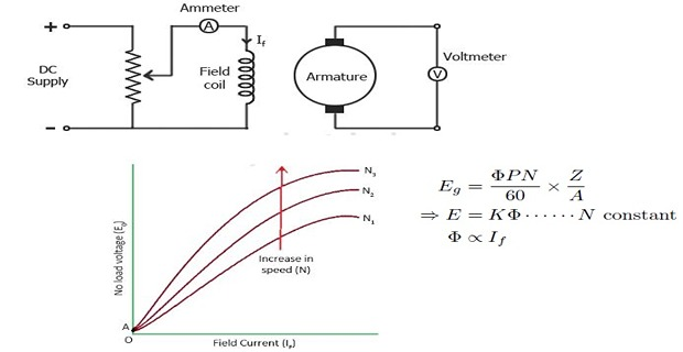
Chapter 28 treated this curve in detail — its residual offset, its straight initial portion, its saturation, and the critical resistance and critical speed that follow from its slope at the origin. The two recapitulations below are given because they bear directly on the characteristics that follow.
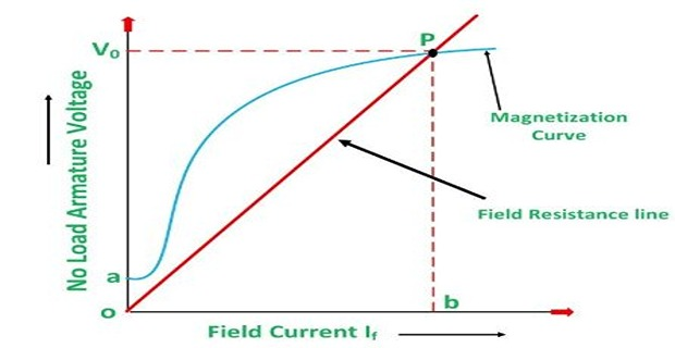
A positive-feedback loop, limited by saturation and started by residual flux, with \(E_g = K\Phi_{res}N\) giving one or two volts to begin.
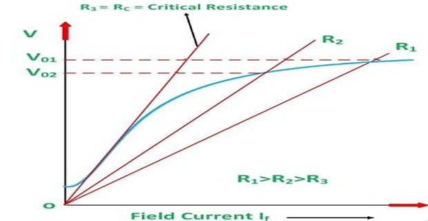
A decrease in \(R_f\) reduces the slope of the \(R_f\) line, giving a higher voltage, and vice versa. If \(R_f\) is raised to \(R_c\) the line becomes tangent to the initial part of the curve; above \(R_c\) the generator fails to excite. Likewise at the critical speed \(N_c\) the line becomes tangential, and below \(N_c\) the voltage will not build up.
Internal Characteristic
It is the relation between the EMF \(E\) actually induced in the armature — that is, after the demagnetising effect of armature reaction — and the armature current \(I_a\).
This characteristic is mainly of interest to the designer.
With no armature reaction the generated voltage would be a horizontal straight line at \(E_0\), since a separately excited machine's flux and speed are both held constant.
In practice there is a voltage drop \(\Delta V_{AR}\) because of armature reaction, which grows with armature current, so the internal characteristic droops.
Chapter 30 explains the mechanism. In outline: the armature current sets up its own mmf on the quadrature axis, which distorts the main field, and because the machine is worked past the knee of its magnetisation curve, the flux gained on one pole tip is less than the flux lost on the other. The net effect is demagnetising, and it grows with load.
External Characteristic
Also called the performance characteristic or voltage-regulating curve.
It is the relation between the terminal voltage \(V\) and the load current \(I\).
It is of great importance in judging the suitability of a generator for a practical purpose.
The external characteristic therefore lies below the internal one by the resistive drop, and both lie below the no-load line by the armature-reaction drop.
The Separately Excited Generator
This is the simplest case, because the field current — and hence \(E_0\) — is held constant by an external supply whatever the load does.

Problem. A separately excited generator has a no-load EMF of 250 V at constant speed and excitation. Armature reaction reduces the induced EMF by \(0.05I_a\) volts, and the armature resistance is 0.15 \(\Omega\). Tabulate the internal and external characteristics up to 200 A and find the voltage regulation at that current.
| \(I_a\) (A) | \(\Delta V_{AR}\) (V) | Internal \(E\) (V) | \(I_aR_a\) (V) | External \(V\) (V) |
|---|---|---|---|---|
| 0 | 0 | 250.0 | 0 | 250.0 |
| 50 | 2.5 | 247.5 | 7.5 | 240.0 |
| 100 | 5.0 | 245.0 | 15.0 | 230.0 |
| 150 | 7.5 | 242.5 | 22.5 | 220.0 |
| 200 | 10.0 | 240.0 | 30.0 | 210.0 |
Combined slope. Both effects are proportional to \(I_a\), so
Voltage regulation at 200 A.
Comment. Armature reaction contributes one quarter of the total droop here, and the armature resistance three quarters. In a large machine the proportion reverses, because the armature resistance is made very small while the armature reaction — which depends on ampere-turns, not on resistance — remains substantial. Chapter 31's compensating windings exist precisely for such machines.
Note that both effects are linear in \(I_a\) in this idealisation, so the external characteristic is a straight line of slope 0.20 \(\Omega\). This is often called the machine's effective internal resistance, and it exceeds the measured \(R_a\) because it includes the magnetic effect.
The Operating Point
The external characteristic says what the generator will supply at each current. The load says what current it will draw at each voltage. Both must hold at once.
The operating point \(P\) is the intersection between the generator's external characteristic and the load characteristic, given by the relation
\(P\) gives the operating values of terminal voltage \(V\) and current \(I\).
This is the same graphical device as Chapter 28's field-resistance line, applied to the output instead of the field. A resistive load is a straight line through the origin of slope \(R_L\), and reducing the load resistance flattens the line, moving the operating point to higher current and lower voltage.
Problem. The generator of Example 29.1 supplies a resistive load. Find the terminal voltage and current for (a) \(R_L = 1.5~\Omega\) and (b) \(R_L = 1.0~\Omega\).
Setting up. The generator gives \(V = 250 - 0.20I\); the load requires \(V = IR_L\). Equating:
(a) \(R_L = 1.5~\Omega\).
Check on the generator curve: \(250 - (0.20)(147.1) = 220.6\) V \(\checkmark\)
(b) \(R_L = 1.0~\Omega\).
Comment. Reducing the load resistance by a third has raised the current 42 % and dropped the voltage 5.6 %. The generator behaves exactly like an ideal 250 V source behind 0.20 \(\Omega\) — which is precisely the Thévenin equivalent, and the reason a DC generator can be treated as such a source in a larger circuit calculation.
The Shunt Generator and Breakdown
A shunt generator droops more steeply than a separately excited one, and for an additional reason.
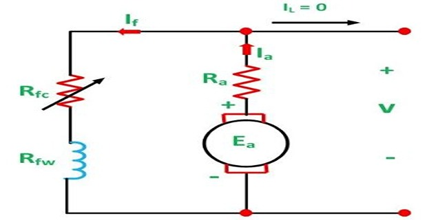
Armature resistance drop \(I_aR_a\), as in any machine.
Armature reaction, weakening the flux.
Reduced field current. The shunt field sees the terminal voltage. As \(V\) falls, \(I_f = V/R_f\) falls, so the flux falls, so \(V\) falls further.
The third is the build-up process of Chapter 28 running in reverse, and it is what gives the shunt generator its distinctive turning-back characteristic.

At the breakdown point the curve turns back on itself. Loading the machine further reduces both the voltage and the current, and on a dead short circuit the terminal voltage is zero, so the shunt field carries no current at all.
The only flux remaining is the residual, so
which is typically a fraction of the rated current. A shunt generator is therefore largely self-protecting against a short circuit — unlike a separately excited machine, whose field is unaffected and whose short-circuit current would be \(E_0/R_a\), possibly thousands of amperes.
Problem. A shunt generator has the external characteristic tabulated below, an armature resistance of 0.15 \(\Omega\) and a residual EMF of 8 V. Identify the breakdown point and estimate the short-circuit current. Compare with a separately excited machine of the same \(E_0 = 250\) V and \(R_a\).
| \(I_L\) (A) | 0 | 50 | 100 | 150 | 200 | 220 | 200 | 150 | 100 |
|---|---|---|---|---|---|---|---|---|---|
| \(V\) (V) | 250 | 240 | 225 | 200 | 160 | 140 | 100 | 60 | 30 |
Breakdown point. The current reaches its greatest value at 220 A, where \(V = 140\) V. Beyond this the curve turns back: at 200 A the voltage has fallen to 100 V, and lower still thereafter.
Short-circuit current. With \(V = 0\) the shunt field is unexcited, so only the residual EMF drives current:
The separately excited comparison. There the field is maintained externally, so \(E_0\) stays at 250 V:
Comment. A factor of 31 between the two. The shunt machine's own feedback saves it: as the terminal voltage collapses the field collapses with it, and the fault current falls to something the winding can survive. The separately excited machine has no such protection and needs a circuit breaker.
Note also that the breakdown current of 220 A is well above the machine's rated load — a generator is not designed to operate anywhere near the turning point, where the characteristic is steep and the voltage unstable.
The Series Generator
Here the field carries the load current, so more load means more flux — and the characteristic rises instead of drooping.

On no load the current is zero, so the flux is only residual and the machine generates a few volts.
As load current rises, \(\Phi \propto I_{se}\) below saturation, so the EMF climbs steeply.
Eventually the field saturates and the EMF levels off, while the resistive drop \(I_a(R_a + R_{se})\) continues to grow linearly.
The external characteristic therefore reaches a maximum and then falls.
Problem. A series generator has the internal characteristic below, with \(R_a + R_{se} = 0.25~\Omega\). Find the external characteristic and the current at which the terminal voltage is greatest.
| \(I\) (A) | 0 | 40 | 80 | 120 | 140 | 160 | 180 |
|---|---|---|---|---|---|---|---|
| \(E\) (V) | 8 | 110 | 178 | 205 | 212 | 217 | 221 |
| \(I(R_a+R_{se})\) | 0 | 10 | 20 | 30 | 35 | 40 | 45 |
| \(V\) (V) | 8 | 100 | 158 | 175 | 177 | 177 | 176 |
The peak. The terminal voltage reaches 177 V and stays there between 140 A and 160 A, then begins to fall.
Why. Differentiating conceptually, the voltage peaks where the rate of rise of the internal EMF equals the rate of rise of the resistive drop:
Between 140 A and 160 A the EMF rises by only 5 V, a slope of \(5/20 = 0.25\) V/A — exactly the resistance. \(\checkmark\)
Comment. The condition is exact and easy to remember: the external characteristic of a series generator peaks where the slope of its magnetisation curve equals its total circuit resistance. Below that current the machine is gaining more from saturation than it loses in resistance; above it, the reverse.
Note the no-load value of 8 V. A series generator cannot excite itself without a load, which is why one is never left open-circuited when in use — and why it must be started with the load already connected.
Compound Generators
A compound machine has both windings, so the drooping shunt characteristic and the rising series characteristic are superimposed. The designer chooses the balance by the number of series turns.
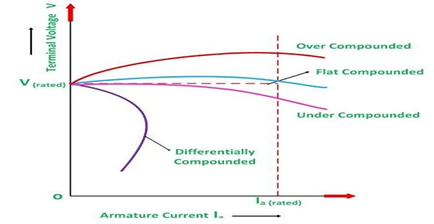
Depending upon the number of series turns \(N_{se}\), a cumulative compound generator can be over-, flat- or under-compounded. If the series-winding ampere-turns are adjusted so that as \(I_L\) increases:
\(V_T\) also increases \(\Rightarrow\) over-compounded
\(V_T\) remains constant \(\Rightarrow\) flat-compounded
If \(N_{se}\) is less than required to be flat-compounded, the generator is said to be under-compounded
In a differentially compounded machine, \(V_T\) falls steeply as \(I_a\) increases, because the series field opposes the shunt field.
Problem. A shunt generator gives 250 V on no load and 230 V at its full load of 100 A. Near the operating point the magnetisation curve has a slope of 40 V per ampere of field current, and the shunt winding has 1200 turns per pole. How many series turns per pole are needed to make it flat-compounded?
The deficit to be made up.
Equivalent extra field current. Using the local slope of the magnetisation curve:
Extra ampere-turns needed per pole.
Series turns. The series winding carries the full load current of 100 A:
Comment. Six turns against the shunt winding's twelve hundred — a ratio of 200 to 1. This is why the series winding is a few turns of heavy strip while the shunt winding is thousands of turns of fine wire: they produce comparable ampere-turns from currents differing by a similar factor.
A machine wound with fewer than six turns would be under-compounded and with more, over-compounded. Because the count must be a whole number, exact flat compounding is rarely achieved; makers commonly fit a slightly generous winding and shunt part of the load current past it with a diverter resistor, which allows fine adjustment on site.
Comparison and Selection
| Type | Shape of \(V\)–\(I\) | Regulation | Short-circuit current | Typical use |
|---|---|---|---|---|
| Separately excited | Straight, gently drooping | Small, positive | Very large | Ward-Leonard, test supplies |
| Shunt | Droops, then turns back | Moderate, positive | Small | Lighting, charging, exciters |
| Series | Rises, peaks, then falls | Large and negative | Large | Boosters only |
| Cumulative, under | Droops slightly | Small, positive | Moderate | General service |
| Cumulative, flat | Level | Zero | Moderate | Nearby loads |
| Cumulative, over | Rises | Negative | Moderate | Long feeders |
| Differential | Falls steeply | Very large | Small | Arc welding |
Summary and Key Formulas
The no-load or open-circuit characteristic relates \(E_0\) to \(I_f\) at fixed speed. It is the magnetisation curve of the pole material and is practically the same shape for all generators.
The internal characteristic relates \(E\) to \(I_a\) after armature reaction, and is of interest to the designer.
The external characteristic relates \(V\) to \(I\) and decides the generator's suitability for a purpose.
\(V = E_0 - \Delta V_{AR} - I_aR_a - 2v_b\). Without armature reaction the internal characteristic would be a horizontal line.
The operating point is where the external characteristic meets the load line \(V_L = I_LR_L\).
A shunt generator droops for three reasons, the third being the fall in field current as \(V\) falls. Past the breakdown point the curve turns back, and the short-circuit current is only \(E_{res}/R_a\) — the machine is largely self-protecting.
A series generator rises with load until saturation, then peaks where \(\mathrm{d}E/\mathrm{d}I = R_a + R_{se}\), then falls. It cannot excite on no load.
Compound machines may be over-, flat- or under-compounded according to the series turns, or differentially compounded for a steeply drooping characteristic.
Flat compounding needs \(N_{se} = \Delta I_f N_{sh}/I_L\) series turns per pole, where \(\Delta I_f\) is the equivalent extra field current.
| Quantity | Relation | Notes |
|---|---|---|
| Internal characteristic | \(E = E_0 - \Delta V_{AR}\) | after armature reaction |
| External characteristic | \(V = E - I_aR_a - 2v_b\) | add \(R_{se}\) if present |
| Effective internal resistance | \(R_{\text{eff}} = R_a + \dfrac{\Delta V_{AR}}{I_a}\) | slope of the external curve |
| Load line | \(V_L = I_LR_L\) | through the origin |
| Operating current | \(I = \dfrac{E_0}{R_L + R_{\text{eff}}}\) | for a linear characteristic |
| Shunt short-circuit current | \(I_{sc} = \dfrac{E_{res}}{R_a}\) | small — self-protecting |
| Sep. excited short circuit | \(I_{sc} = \dfrac{E_0}{R_a}\) | very large |
| Series generator peak | \(\dfrac{\mathrm{d}E}{\mathrm{d}I} = R_a + R_{se}\) | condition for maximum \(V\) |
| Series turns for flat compounding | \(N_{se} = \dfrac{\Delta I_f N_{sh}}{I_L}\) | \(\Delta I_f = \Delta V/(\mathrm{d}E/\mathrm{d}I_f)\) |
| Voltage regulation | \(\dfrac{V_{NL} - V_{FL}}{V_{FL}} \times 100\,\%\) | negative if over-compounded |
Common Mistakes
Confusing the internal and external characteristics. Internal plots \(E\) against \(I_a\); external plots \(V\) against \(I\), and the two differ by the resistive drop.
Plotting the external characteristic against \(I_a\). In a shunt machine \(I \ne I_a\) — the field current must be subtracted.
Forgetting the third cause of droop in a shunt machine. The falling terminal voltage weakens the field, which is what produces the turning-back.
Expecting a large short-circuit current from a shunt generator. It is only \(E_{res}/R_a\), because the field dies with the voltage.
Applying that reasoning to a separately excited machine. Its field is unaffected and its fault current is enormous.
Treating the breakdown point as a normal operating condition. It lies well beyond rated load and the characteristic there is steep and unstable.
Assuming a series generator's voltage rises indefinitely. It peaks where the magnetisation slope equals the circuit resistance.
Trying to run a series generator on no load. With no current there is no field and only the residual voltage appears.
Confusing over-compounding with over-excitation. Over-compounding means the series turns give a rising characteristic; it says nothing about the shunt field setting.
Thinking a negative regulation is a fault. An over-compounded generator is designed to produce it.
Chapter Review
Decide first which characteristic is wanted, and whether the current on the axis is \(I_a\) or \(I_L\).
P29.1 A separately excited generator has \(E_0 = 300\) V, an armature-reaction drop of \(0.04I_a\) volts and \(R_a = 0.12~\Omega\). Find the terminal voltage at 150 A and the regulation.
Show answer
\[V = 300 - (0.04 + 0.12)(150) = 300 - (0.16)(150) = 300 - 24 = 276~\mathrm{V}\]\[\text{regulation} = \frac{300 - 276}{276} = 8.70\,\%\]P29.2 The generator of P29.1 feeds a 2.0 \(\Omega\) resistive load. Find the operating point.
Show answer
\[I = \frac{300}{2.0 + 0.16} = \frac{300}{2.16} = 138.9~\mathrm{A}, \qquad V = (138.9)(2.0) = 277.8~\mathrm{V}\]P29.3 A shunt generator has \(R_a = 0.10~\Omega\) and a residual EMF of 10 V. Estimate its short-circuit current, and compare with a separately excited machine of the same \(R_a\) generating 240 V.
Show answer
\[I_{sc,\text{shunt}} = \frac{10}{0.10} = 100~\mathrm{A}\]A factor of 24. The shunt machine's field collapses with the voltage; the separately excited machine's does not.\[I_{sc,\text{sep}} = \frac{240}{0.10} = 2400~\mathrm{A}\]P29.4 A series generator has \(R_a + R_{se} = 0.30~\Omega\). Between 100 A and 120 A its EMF rises from 190 V to 196 V. Is the terminal voltage still rising?
Show answer
This equals \(R_a + R_{se}\), so the terminal voltage is at its maximum over this interval. Checking: \(V(100) = 190 - 30 = 160\) V and \(V(120) = 196 - 36 = 160\) V \(\checkmark\)\[\frac{\mathrm{d}E}{\mathrm{d}I} = \frac{196 - 190}{120 - 100} = \frac{6}{20} = 0.30~\mathrm{V/A}\]P29.5 A shunt generator gives 220 V no-load and 205 V at 80 A full load. The magnetisation slope is 50 V/A and the shunt winding has 1000 turns per pole. Find the series turns for flat compounding.
Show answer
\[\Delta V = 15~\mathrm{V}, \qquad \Delta I_f = \frac{15}{50} = 0.30~\mathrm{A}\]So 4 turns per pole, rounded up — giving slight over-compounding, which a diverter resistor can trim back.\[\Delta(NI) = (0.30)(1000) = 300~\mathrm{AT/pole}, \qquad N_{se} = \frac{300}{80} = 3.75\]P29.6 Why does the internal characteristic of a separately excited generator droop at all, when its field current and speed are both constant?
Show answer
Because of armature reaction. The armature current sets up its own mmf, which distorts the main field. Since the machine works past the knee of its magnetisation curve, the flux gained at one pole tip is less than the flux lost at the other, so the net flux falls.The effect grows with armature current, so the induced EMF falls below \(E_0\) by an amount \(\Delta V_{AR}\) that increases with load. Without armature reaction the internal characteristic would be a horizontal straight line.
P29.7 Explain the turning-back of a shunt generator's external characteristic.
Show answer
Up to the breakdown point, reducing the load resistance increases the current. But the terminal voltage falls, and since the shunt field sees that voltage, the field current and hence the flux fall too.Beyond a certain point the loss of flux outweighs the reduction in load resistance, so the current begins to fall as well as the voltage. This is Chapter 28's build-up loop running in reverse — a collapse rather than a build-up. The curve therefore doubles back and meets the current axis at the small short-circuit value \(E_{res}/R_a\).
P29.8 A generator is required to hold constant voltage at a load 500 m away. Which type, and why not a flat-compounded machine?
Show answer
An over-compounded machine. Its terminal voltage rises with load, and the rise is designed to match the \(IR\) drop in the cable so that the voltage at the far end stays constant.A flat-compounded machine holds its own terminals constant, which means the load at the far end sees a voltage falling with current. The customer is at the far end, not at the generator.
P29.9 Why is the external characteristic the one that matters commercially?
Show answer
It is the only one that can be measured at the terminals and the only one the load experiences. The no-load characteristic requires the armature to be open-circuited, and the internal characteristic involves an EMF that exists inside the winding and cannot be reached by a voltmeter.The external characteristic answers the customer's question directly: how much will the voltage sag when I draw current? That is what determines whether the machine suits the duty.
P29.10 A series generator is started with its load disconnected and produces almost nothing. Is it faulty?
Show answer
No — it is behaving exactly as it must. The field winding carries the load current, so with no load there is no field current, no flux beyond the residual, and therefore only a few volts.A series generator must be started with its load connected. This is the mirror image of the series motor rule from Chapter 20: a series motor must never run unloaded, and a series generator must never be excited unloaded — both because the field and the load current are the same thing.
MCQ 1. The open-circuit characteristic plots:
(a) \(V\) against \(I\) (b) \(E_0\) against \(I_f\) (c) \(E\) against \(I_a\) (d) \(I_f\) against \(I_a\)Show answer
(b) \(E_0\) against \(I_f\) at a fixed speed.MCQ 2. The internal characteristic differs from the no-load line because of:
(a) armature resistance (b) armature reaction (c) brush drop (d) frictionShow answer
(b) armature reaction, which demagnetises the main field.MCQ 3. The characteristic of most interest to the user is the:
(a) no-load (b) internal (c) external (d) magnetisationShow answer
(c) external — the voltage-regulating curve.MCQ 4. The operating point is the intersection of the external characteristic with the:
(a) OCC (b) field-resistance line (c) load line (d) internal characteristicShow answer
(c) load line, \(V_L = I_LR_L\).MCQ 5. The short-circuit current of a shunt generator is:
(a) very large (b) small, set by residual EMF (c) zero (d) equal to rated currentShow answer
(b) small, set by residual EMF, since the field collapses with the terminal voltage.MCQ 6. Beyond the breakdown point of a shunt generator:
(a) current rises, voltage falls (b) both fall (c) both rise (d) voltage risesShow answer
(b) both fall — the curve turns back on itself.MCQ 7. The external characteristic of a series generator peaks where:
(a) \(E = V\) (b) \(\mathrm{d}E/\mathrm{d}I = R_a + R_{se}\) (c) the field saturates (d) \(I = 0\)Show answer
(b) \(\mathrm{d}E/\mathrm{d}I = R_a + R_{se}\) — where the EMF gain just matches the resistive loss.MCQ 8. A flat-compounded generator has a full-load voltage:
(a) above no-load (b) equal to no-load (c) below no-load (d) zeroShow answer
(b) equal to no-load, giving zero regulation.MCQ 9. If \(N_{se}\) is less than needed for flat compounding, the machine is:
(a) over-compounded (b) under-compounded (c) differentially compounded (d) separately excitedShow answer
(b) under-compounded — the voltage still droops, but less than a plain shunt machine.MCQ 10. In a differentially compounded generator, as \(I_a\) increases the terminal voltage:
(a) rises (b) stays constant (c) falls steeply (d) falls slightlyShow answer
(c) falls steeply, since the series field opposes the shunt field.
Define the three characteristics of a DC generator and say who uses each and why.
Explain why the internal characteristic droops even at constant field current and speed.
Explain how the operating point is located, and what happens to it as the load resistance falls.
Give the three causes of droop in a shunt generator and identify which produces the turning-back.
Explain why the short-circuit current of a shunt generator is small but that of a separately excited machine is not.
Account for the rise, peak and fall of a series generator's external characteristic.
Distinguish over-, flat-, under- and differentially compounded machines and give an application of each.
Outline how the number of series turns for flat compounding is calculated.
Armature reaction has been used repeatedly in this chapter but never explained. Chapter 30 supplies it: how the armature's own mmf, acting on the quadrature axis, distorts the main field, why the net effect is demagnetising once the iron is past its knee, and how the demagnetising and cross-magnetising ampere-turns are calculated.
Chapter 30 also shows that armature reaction shifts the magnetic neutral axis away from the geometrical neutral plane — which invalidates the assumption of Chapter 23 that the commutating coil sits where its EMF is zero. Chapter 31 then deals with the consequences under the heading of commutation, and with the two remedies that make large DC machines possible: interpoles and compensating windings.