By the end of this chapter you should be able to:
Explain why magnetic circuits are excited from AC rather than DC, and what inductance contributes in each case.
State the reversal of cause and effect between DC and AC excitation, and use it to predict what is fixed and what adjusts.
Derive the EMF equation \(E = 4.44 f N \Phi_m\) both by differentiation and by the form-factor route.
Establish the phase relationship between flux, induced EMF, applied voltage and exciting current.
Resolve the exciting current into its magnetising and core-loss components from no-load test data.
Explain why a sinusoidal flux demands a peaky, non-sinusoidal magnetising current, and identify the dominant harmonic.
Draw the shunt equivalent circuit and compute \(R_0\) and \(X_m\).
Explain volts-per-hertz operation and why \(B_m\) depends on \(V/f\) rather than on \(V\) alone.
Introduction
To magnetise the magnetic circuits of electrical devices such as transformers, AC machines and electromagnetic relays, an AC supply is used. The magnetisation of a magnetic circuit is called its excitation.
Chapters 2 to 7 treated the magnetic circuit as a static object: given a current, find the flux; given a flux, find the loss. This chapter sets it in motion. Once the excitation alternates, three new things happen at once. The flux induces an EMF that opposes the supply, so the voltage rather than the current comes to control the flux. The core's non-linearity distorts the current waveform. And the losses of Chapters 6 and 7 must be drawn from the supply as a real, in-phase component of current.
Everything in this chapter reappears almost unchanged in Chapter 41, where the same analysis is applied to a transformer, and again in Chapter 58 for the induction motor. The EMF equation derived in Section 8-3 is arguably the most-used single formula in the whole book.
DC versus AC Excitation
Magnetic circuits are essentially never excited by a DC supply, and the reason repays careful attention because it establishes the logic of everything that follows.
Under DC excitation, the steady-state current is determined by the impressed voltage and the resistance of the circuit alone:
The coil inductance \(L_{\text{coil}}\) comes into the picture only during the transient period — that is, while the current is building up or decaying at the switching instants. Once the transient has died away, the inductor is simply a piece of wire. The flux then adjusts itself in accordance with the steady-state current, so that the relationship imposed by the magnetisation (B–H) curve is satisfied.
Under AC excitation, inductance comes into the picture even in the steady state, because the flux never stops changing. As a result, for most magnetic circuits — though not for all — the flux is determined by the impressed voltage and frequency. The magnetising current then adjusts itself in accordance with this flux, so that the relationship imposed by the magnetisation curve is satisfied.
Under DC: voltage and resistance fix the current; the B–H curve then determines the flux.
Under AC: voltage and frequency fix the flux; the B–H curve then determines the current.
The B–H curve is consulted in both cases, but it is read in opposite directions. Recognising which quantity is imposed and which adjusts will resolve most of the confusion students meet in transformer theory.
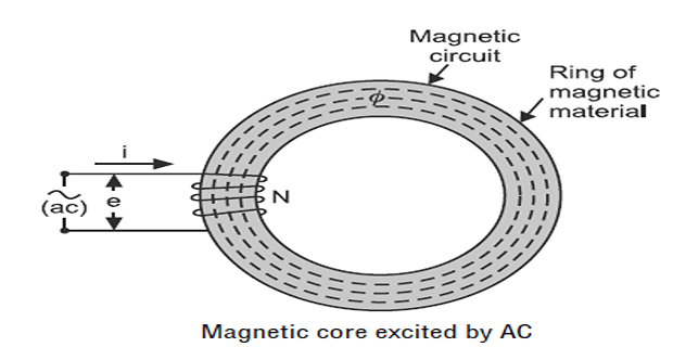
For economic reasons the normal working flux density is kept beyond the linear portion of the magnetisation curve — pushing the iron hard keeps the core small, as Chapter 6 showed. A consequence is that an accurate value of self-inductance cannot be predicted, because \(L = N^{2}/S\) and the reluctance depends on the operating point.
Nevertheless, for all practical purposes the parameters of the magnetic circuit are treated as constant, and a single value of \(X_m\) is used in the equivalent circuit. This is an approximation, adopted knowingly, and it works because — as the diagram above stresses — the core's non-linearity affects the current rather than the flux, and the current is a small quantity at no load.
The EMF Equation
This is the central result of the chapter. Assume the flux is sinusoidal — which, as Section 8-2 argued, is what the impressed sinusoidal voltage enforces.
By Faraday's law the EMF induced in the \(N\)-turn coil is
The peak value is therefore
and, since the waveform is sinusoidal, the RMS value is
The constant 4.44 is \(2\pi/\sqrt{2} = \pi\sqrt{2}\), and it carries a hidden assumption: the waveform is sinusoidal. Section 8-6 and Worked Example 8.5 show what happens when it is not.
This route avoids calculus and shows exactly where the 4.44 comes from, which is worth seeing at least once.
In one quarter of a cycle the flux rises from zero to \(\Phi_m\), taking a time \(T/4 = 1/4f\). The average rate of change is therefore
For a sine wave the form factor — the ratio of RMS to average — is
Written this way the general form is \(E = 4 k_f f N \Phi_m\). The familiar 4.44 is simply \(4 \times 1.11\), and it must be replaced whenever the supply is not sinusoidal.
Problem. A coil of 500 turns is wound on a core of cross-section 40 cm² and connected to a 230 V, 50 Hz supply. Neglecting the resistance drop, find the maximum flux, the maximum flux density, and the peak induced EMF.
Maximum flux. With \(E \approx V\):
Maximum flux density.
Peak EMF.
Check against \(E_m = 2\pi f N \Phi_m = 2\pi(50)(500)\left(2.072\times10^{-3}\right) = 325.5\) V \(\checkmark\)
Comment. Note again what did not enter the calculation: the material of the core, its permeability, its mean length, and whether it contains an air gap. The flux density is set entirely by the supply and the winding. A designer wanting a higher \(B_m\) must reduce the turns or the area, not change the steel.
Problem. The coil of Example 8.1 has a resistance of 8 \(\Omega\), and its core has a mean length of 0.6 m with \(\mu_r = 3000\). Compare the current and the copper loss when the coil is connected to (a) 230 V DC and (b) 230 V, 50 Hz AC.
(a) DC supply. In the steady state only the resistance limits the current:
The mmf this implies is \((28.75)(500) = 14\,375\) AT, giving \(H = 14\,375/0.6 = 23\,958\) AT/m. If the iron were linear, the flux density would be
which is of course impossible — the core saturates at about 2 T and stays there. The current is not limited by the magnetic circuit at all; the coil simply dissipates 6.6 kW and burns out within seconds.
(b) AC supply. From Example 8.1, \(B_m = 0.518\) T, so
Comment. The copper loss differs by a factor of about 60,000. Under AC the induced EMF opposes the supply almost entirely, and the coil draws only the small current needed to magnetise the core; under DC there is no induced EMF in the steady state and nothing but 8 \(\Omega\) of copper stands between the supply and the winding. This is the whole reason magnetic circuits are excited from AC — and the reason a transformer connected to DC destroys itself.
Phase Relationships
Equations (i) and (ii) of Section 8-3 reveal that the induced EMF leads the flux — and hence the exciting current — by \(\pi/2\) radians, or 90°. This follows directly from differentiating a sine to obtain a cosine.
The supply voltage must overcome two things: the induced EMF and the resistance drop of the coil. In electrical machines the drop in \(R\) is usually only a few percent of \(V\) and is therefore neglected, so \(E\) and \(V\) may be considered equal in magnitude:
Two conventions are in common use, and they differ by a sign. Writing \(e = +N\,\mathrm{d}\Phi/\mathrm{d}t\), as above, makes the EMF lead the flux by 90°. Writing \(e = -N\,\mathrm{d}\Phi/\mathrm{d}t\) — emphasising Lenz's law — makes it lag by 90°. The physics is identical; only the reference direction differs.
This book follows the first convention here and in Chapter 41. What matters, and is convention-independent, is that flux and EMF are in quadrature, and that the exciting current is very nearly in phase with the flux.
Components of the Exciting Current
If the core were lossless, the exciting current would be purely reactive — in phase with the flux, and therefore 90° out of phase with the voltage, drawing no real power. Real cores are not lossless: the hysteresis and eddy-current losses of Chapters 6 and 7 must be paid for, and the payment can only come from the supply as real power.
The exciting current (also called the no-load current) therefore has two components:
In phase with the flux, and hence lagging the voltage by 90°. It produces the flux and draws no real power. This is the larger component, typically 95–98 % of \(I_0\).
In phase with the applied voltage. Also called the working, active or wattful component. It supplies the hysteresis and eddy-current losses.
The no-load power factor \(\cos\phi_0\) is characteristically poor — 0.1 to 0.3 — because \(I_m\) so greatly exceeds \(I_c\). This is not a defect: the current itself is only a few percent of full-load current, so the reactive burden is small in absolute terms. It becomes significant only for lightly loaded transformers left permanently energised.
Problem. A coil wound on a laminated core takes 0.8 A from a 230 V, 50 Hz supply on no load, and the wattmeter reads 45 W. Find the no-load power factor, the two components of the exciting current, and the parameters \(R_0\) and \(X_m\) of the shunt branch.
No-load power factor.
so \(\phi_0 = 75.85^{\circ}\) and \(\sin\phi_0 = 0.9696\).
Components.
Check: \(\sqrt{0.1957^{2} + 0.7757^{2}} = \sqrt{0.0383 + 0.6017} = 0.800\) A \(\checkmark\)
Shunt parameters.
Cross-check: \(R_0 = V^{2}/P_0 = 230^{2}/45 = 1176~\Omega\) \(\checkmark\)
Comment. The 45 W is the core loss — hysteresis plus eddy currents — because the copper loss at 0.8 A is negligible. This is exactly the reasoning behind the transformer open-circuit test of Chapter 46, and the numbers obtained here are precisely the shunt-branch parameters used there. The measurement separates the two components without any knowledge of the core's material or geometry.
Waveform Distortion
Here the non-linearity of Chapter 5 makes itself felt in a new way. The supply voltage forces the flux to be sinusoidal. But the relationship between flux and current is the B–H curve, which is not a straight line. A sinusoidal flux therefore requires a non-sinusoidal current.
The shape is easy to predict. Near the peak of the flux wave the core is approaching saturation, where a large increase in \(H\) produces very little increase in \(B\). To hold the flux on its sinusoidal path through the peak, the current must rise disproportionately. The result is a peaky waveform: flatter than a sine near the zero crossings, and sharply pointed at the maxima.
A Fourier analysis of this waveform shows a strong third harmonic, typically 30–40 % of the fundamental in a core worked near saturation, together with smaller fifth and seventh components. Even harmonics are absent because the waveform has half-wave symmetry.
In a balanced three-phase system the fundamentals are 120° apart, but the third harmonics are \(3\times120^{\circ} = 360^{\circ}\) apart — that is, in phase with one another. They therefore cannot cancel at the star point; they add. If no path is provided, the flux waveform distorts instead and dangerous peak voltages can appear.
The standard remedies are a delta-connected winding or a delta tertiary, which give the third-harmonic currents a closed path in which to circulate. Chapter 54 treats this properly; it is the main reason three-phase transformer connections are chosen as they are.
Hysteresis adds asymmetry. If hysteresis as well as saturation is included, the current waveform is no longer symmetrical about its own peak: it reaches its maximum slightly before the flux does, because the descending branch of the loop lies above the ascending one. This forward tilt is the waveform-level expression of the core-loss component \(I_c\) identified in Section 8-5.
The Shunt Equivalent Circuit
For circuit analysis it is convenient to replace the whole magnetic circuit by two elements in parallel across the supply, each carrying one component of the exciting current.
A fictitious resistance that dissipates exactly the hysteresis and eddy-current losses. No such resistor exists physically — the heat appears in the iron, not in a component.
Represents the energy stored and returned each cycle. Large when the core is permeable, small when it is not — and, strictly, not constant, since the core is non-linear.
This shunt branch is precisely what appears in the transformer equivalent circuit of Chapter 44, and — with one resistance made slip-dependent — in the induction-motor equivalent circuit of Chapter 64. It is worth being comfortable with it now.
Problem. A transformer is designed for 400 V, 50 Hz, at which \(B_m = 1.4\) T. Find the flux density when it is operated at (a) 400 V, 60 Hz; (b) 400 V, 40 Hz; (c) 440 V, 50 Hz; (d) 440 V, 55 Hz. Comment on each.
Principle. From the EMF equation, with \(N\) and \(A\) fixed,
| Case | \(V\) | \(f\) | \(V/f\) | \(B_m\) | Verdict |
|---|---|---|---|---|---|
| Rated | 400 | 50 | 8.00 | 1.400 T | Design point |
| (a) | 400 | 60 | 6.67 | 1.167 T | Safe — less flux, less core loss |
| (b) | 400 | 40 | 10.00 | 1.750 T | Deep saturation — dangerous |
| (c) | 440 | 50 | 8.80 | 1.540 T | Over-excited — past the knee |
| (d) | 440 | 55 | 8.00 | 1.400 T | Unchanged — \(V/f\) preserved |
Comment. Case (b) is the important one. A transformer rated for 60 Hz and connected to a 50 Hz supply at the same voltage sees its flux density rise by 20 %; a 50 Hz unit on 40 Hz sees 25 %. Either drives the core well past the knee, where the magnetising current rises steeply and becomes violently peaky. Case (d) shows the remedy: raise the voltage and the frequency together, keeping \(V/f\) constant, and the flux density does not change at all.
This is the principle of V/f control, the standard method of varying the speed of an induction motor (Chapter 68). Holding \(V/f\) constant keeps the machine's flux — and therefore its torque capability — unchanged across the whole speed range.
Inrush Current
One consequence of AC excitation deserves mention now, though Chapter 50 treats it fully. It concerns the instant of switching on.
In the steady state the flux lags the voltage by 90°, so when the voltage is at its zero crossing the flux is at its negative peak. If the supply is switched on at a voltage zero, the flux must start from whatever value it happens to have — typically the residual \(B_r\) — and integrate upward from there. Over the first half cycle it therefore rises by the full \(2\Phi_m\) instead of swinging symmetrically about zero:
A core designed to work at 1.4 T is thus asked to carry something over 2.8 T, which is far beyond saturation. Its reluctance collapses to essentially that of an air-cored coil, and the current required becomes enormous — commonly 8 to 12 times rated current for the first few cycles, decaying over several hundred milliseconds as winding resistance damps the transient.
Problem. A transformer designed for a sinusoidal 230 V, 50 Hz supply operates at \(B_m = 1.30\) T. It is instead fed from a square-wave inverter of the same RMS voltage and frequency. Find the new flux density and comment.
Principle. The general EMF equation is \(E = 4 k_f f N \Phi_m\), so at fixed \(E\), \(f\) and \(N\):
Form factors. For a sine wave \(k_f = 1.11\); for a square wave the RMS and average values are equal, so \(k_f = 1.00\).
Comment. An 11 % rise in flux density, produced with no change whatever in RMS voltage or frequency. For a core already worked at 1.30 T this may be enough to push it past the knee, raising the magnetising current sharply and the core loss with it.
The moral is that "230 V, 50 Hz" does not by itself determine the flux — the waveform matters too. This is why transformers fed from square-wave or modified-sine inverters run hotter than the same units on a sinusoidal mains, and why inverter-duty transformers are derated. It is also why the 4.44 in the EMF equation should be remembered as \(4k_f\), with the 1.11 made explicit.
Applications
The EMF equation fixes the turns-per-volt from the core area and the chosen working flux density. Every transformer design begins here, and Chapter 41 does exactly this calculation.
Energising a transformer on no load and measuring \(V\), \(I_0\) and \(P_0\) yields the core loss and the shunt parameters directly, exactly as in Worked Example 8.3. Chapter 46 develops the full procedure.
Holding the volts-per-hertz ratio constant maintains flux and hence torque capability as the frequency is varied. This single idea underlies almost every variable-speed AC drive in service (Chapter 68).
The third-harmonic magnetising current of Section 8-6 must be given a circulating path. This determines the choice between star, delta and star–delta–tertiary arrangements (Chapters 52–54).
An AC-operated relay draws a large current when its armature is open (high reluctance, low \(X_m\)) and much less once it has closed. This gives a natural high pull-in and low hold current — one reason AC coils need no economy resistor.
Inrush current forces overcurrent relays to be time-delayed or harmonic-restrained on transformer feeders, since a healthy energisation looks momentarily like a fault.
Summary and Key Formulas
The magnetisation of a magnetic circuit is called its excitation, and AC supply is used for transformers, AC machines and relays.
Under DC, the steady current is \(V/R\) and inductance matters only during transients; the flux then adjusts to satisfy the B–H curve.
Under AC, inductance acts in the steady state, the flux is fixed by the impressed voltage and frequency, and the current adjusts to satisfy the B–H curve. Cause and effect are exchanged.
The EMF equation is \(E = 4.44 f N \Phi_m = 4.44 f N B_m A\), where 4.44 \(= 4k_f\) assumes a sinusoidal waveform.
The induced EMF leads the flux — and the exciting current — by 90°. The resistance drop is small, so \(E \approx V\).
The exciting current splits into \(I_m\) (magnetising, in phase with flux) and \(I_c\) (core loss, in phase with voltage). The no-load power factor is poor, 0.1 to 0.3.
A sinusoidal flux requires a peaky, non-sinusoidal current rich in third harmonic, which must be given a circulating path in three-phase systems.
\(B_m \propto V/f\). Holding volts per hertz constant holds the flux density constant — the basis of variable-speed drive control.
Switching on at a voltage zero can drive the flux to \(2\Phi_m + \Phi_r\), producing an inrush current of 8 to 12 times rated.
| Quantity | Formula | Notes |
|---|---|---|
| Sinusoidal flux | \(\Phi = \Phi_m\sin 2\pi f t\) | imposed by the supply |
| Induced EMF | \(e = N\dfrac{\mathrm{d}\Phi}{\mathrm{d}t} = 2\pi f N\Phi_m\cos 2\pi ft\) | leads flux by 90° |
| Peak EMF | \(E_m = 2\pi f N \Phi_m\) | volts |
| EMF equation | \(E = 4.44 f N \Phi_m\) | RMS; sinusoidal only |
| In terms of \(B\) | \(E = 4.44 f N B_m A\) | design form |
| General form | \(E = 4 k_f f N \Phi_m\) | \(k_f = 1.11\) for a sine |
| Average EMF | \(E_{\text{av}} = 4 f N\Phi_m\) | over a quarter cycle |
| Flux density | \(B_m = \dfrac{V}{4.44 f N A}\) | \(B_m \propto V/f\) |
| Exciting current | \(I_0 = \sqrt{I_m^{2} + I_c^{2}}\) | no-load current |
| Core-loss component | \(I_c = I_0\cos\phi_0 = \dfrac{P_0}{V}\) | in phase with \(V\) |
| Magnetising component | \(I_m = I_0\sin\phi_0\) | in phase with \(\Phi\) |
| No-load power factor | \(\cos\phi_0 = \dfrac{P_0}{V I_0}\) | typically 0.1 to 0.3 |
| Core-loss resistance | \(R_0 = \dfrac{V}{I_c} = \dfrac{V^{2}}{P_0}\) | shunt branch |
| Magnetising reactance | \(X_m = \dfrac{V}{I_m} = 2\pi f L_m\) | shunt branch |
| Inrush flux | \(\Phi_{\text{peak}} \approx 2\Phi_m + \Phi_r\) | switching at voltage zero |
Common Mistakes
Thinking the core material determines the flux under AC. It does not. \(B_m = V/(4.44fNA)\) contains no material property whatever. The core determines the current needed.
Applying \(I = V/R\) to an AC-excited coil. That is the DC result. Under AC the induced EMF, not the resistance, limits the current — by a factor of tens of thousands, as Example 8.2 showed.
Using 4.44 for a non-sinusoidal supply. The constant is \(4k_f\). For a square wave it is 4.00, and the flux is 11 % higher for the same RMS voltage.
Confusing \(\Phi_m\) with an RMS flux. The EMF equation uses the maximum flux. There is no such thing as an RMS flux in this formula.
Assuming \(B_m\) depends on voltage alone. It depends on \(V/f\). Raising both together leaves it unchanged.
Swapping \(I_m\) and \(I_c\). The magnetising component is in phase with the flux; the core-loss component is in phase with the voltage. Only the latter carries real power.
Expecting a good no-load power factor. It is characteristically 0.1 to 0.3, because \(I_m \gg I_c\). That is normal, not a fault.
Assuming the magnetising current is sinusoidal. It cannot be, if the flux is. The equivalent circuit replaces it by an equivalent sinusoid — a knowing approximation.
Believing inrush depends on the load. It is purely magnetic and occurs with the secondary open-circuited. It depends on the point on the wave at which the switch closes and on the residual flux.
Forgetting that \(R_0\) is fictitious. No resistor dissipates the core loss; the heat appears in the iron. \(R_0\) is a circuit-modelling device.
Chapter Review
Assume sinusoidal supply and neglect the resistance drop unless told otherwise.
P8.1 A coil of 800 turns is wound on a core of area 25 cm² working at \(B_m = 1.2\) T, 50 Hz. Find the induced EMF.
Show answer
\[E = 4.44 f N B_m A = (4.44)(50)(800)(1.2)\left(25\times10^{-4}\right) = 532.8~\mathrm{V}\]P8.2 How many turns are needed to induce 240 V at 50 Hz with a maximum flux of 2.5 mWb?
Show answer
Turns must be an integer, so the actual flux will differ very slightly from 2.5 mWb.\[N = \frac{E}{4.44 f \Phi_m} = \frac{240}{(4.44)(50)\left(2.5\times10^{-3}\right)} = \frac{240}{0.555} = 432.4 \ \to\ 432~\text{turns}\]P8.3 A 415 V, 50 Hz supply feeds a 250-turn coil on a core of area 60 cm². Find \(\Phi_m\) and \(B_m\).
Show answer
\[\Phi_m = \frac{415}{(4.44)(50)(250)} = \frac{415}{55\,500} = 7.477\times10^{-3}~\mathrm{Wb}\]\[B_m = \frac{7.477\times10^{-3}}{60\times10^{-4}} = 1.246~\mathrm{T}\]P8.4 A transformer rated 230 V, 50 Hz works at \(B_m = 1.35\) T. What flux density results at 230 V, 25 Hz, and what happens?
Show answer
Since \(B_m \propto V/f\) and the frequency has halved:This is far beyond the saturation density of any steel, so the flux cannot actually reach it. Instead the core saturates violently, the magnetising current rises to many times rated, the waveform becomes extremely peaky, and the transformer overheats within minutes. Halving the frequency at rated voltage is one of the most destructive things that can be done to a transformer.\[B_m' = (1.35)\left(\frac{50}{25}\right) = 2.70~\mathrm{T}\]P8.5 A coil takes 1.2 A at 240 V, 50 Hz on no load, absorbing 60 W. Find \(\cos\phi_0\), \(I_c\), \(I_m\), \(R_0\) and \(X_m\).
Show answer
\[\cos\phi_0 = \frac{60}{(240)(1.2)} = \frac{60}{288} = 0.2083, \qquad \sin\phi_0 = 0.9781\]\[I_c = (1.2)(0.2083) = 0.250~\mathrm{A}, \qquad I_m = (1.2)(0.9781) = 1.174~\mathrm{A}\]Check: \(V^{2}/P_0 = 57\,600/60 = 960~\Omega\) \(\checkmark\)\[R_0 = \frac{240}{0.250} = 960~\Omega, \qquad X_m = \frac{240}{1.174} = 204.5~\Omega\]P8.6 For the coil of P8.5, the core loss splits 60 % hysteresis and 40 % eddy current. Find each, and state which component of \(I_0\) supplies them.
Show answer
Both are supplied by the core-loss component \(I_c = 0.250\) A, which is in phase with the voltage and therefore carries real power. The magnetising component \(I_m = 1.174\) A is in quadrature and carries none — it merely exchanges energy with the field each half cycle.\[P_h = (0.60)(60) = 36~\mathrm{W}, \qquad P_e = (0.40)(60) = 24~\mathrm{W}\]P8.7 A core of mean length 0.5 m and area 5 cm² carries 400 turns and works at \(B_m = 1.11\) T, at which the B–H curve of Chapter 5 gives \(H = 800\) AT/m. Find the peak magnetising current, and its RMS value assuming a sinusoidal approximation.
Show answer
\[\mathcal{F}_m = H l = (800)(0.5) = 400~\mathrm{AT} \quad\Longrightarrow\quad I_m(\text{peak}) = \frac{400}{400} = 1.00~\mathrm{A}\]The sinusoidal assumption is an approximation: the true waveform is peaky, so its RMS value is somewhat lower than \(I_{\text{peak}}/\sqrt{2}\) for the same peak — the waveform spends less time near its maximum than a sine does.\[I_m(\text{rms}) \approx \frac{1.00}{\sqrt{2}} = 0.707~\mathrm{A}\]P8.8 A transformer designed for a sinusoidal supply at \(B_m = 1.25\) T is fed from a square wave of the same RMS voltage and frequency. Find the new \(B_m\).
Show answer
An 11 % increase with no change in RMS voltage. The same RMS voltage does not imply the same flux — the waveform matters.\[B_m' = (1.25)\frac{k_{f,\text{sine}}}{k_{f,\text{square}}} = (1.25)\left(\frac{1.11}{1.00}\right) = 1.388~\mathrm{T}\]P8.9 A transformer has a rated current of 25 A. Estimate the peak inrush current, and state on what it depends.
Show answer
Taking the usual range of 8 to 12 times rated:It depends on the point on the voltage wave at which the switch closes (worst at a voltage zero, least at a peak), on the residual flux left from the previous de-energisation and its polarity, and on the winding resistance which damps the transient. It does not depend on the load.\[I_{\text{inrush}} \approx (8 \text{ to } 12)(25) = 200 \text{ to } 300~\mathrm{A}\]P8.10 A coil is wound on a core and excited from a fixed AC supply. The core is then replaced with one of half the permeability, all dimensions unchanged. What happens to \(B_m\), to \(I_m\) and to \(X_m\)?
Show answer
\(B_m\): unchanged. From \(B_m = V/(4.44fNA)\), no material property appears — the supply and winding fix the flux density.
\(I_m\): doubles. Halving \(\mu\) doubles the reluctance, so twice the mmf is needed for the same flux.
\(X_m\): halves. Since \(X_m = V/I_m\) and \(I_m\) has doubled. Equivalently \(L = N^{2}/S\) has halved.
This is the reversal of Section 8-2 in a single question: the core does not control the flux, only the current required to produce it.
MCQ 1. Under AC excitation the flux in a core is determined by:
(a) the current (b) the impressed voltage and frequency (c) the core material (d) the resistanceShow answer
(b) the impressed voltage and frequency. The current then adjusts to satisfy the B–H curve.MCQ 2. In the EMF equation, the constant 4.44 equals:
(a) \(2\pi\) (b) \(\pi\sqrt{2}\) (c) \(4/\sqrt{2}\) (d) \(\pi/2\)Show answer
(b) \(\pi\sqrt{2} = 2\pi/\sqrt{2} = 4.443\). Equivalently \(4k_f\) with \(k_f = 1.11\).MCQ 3. The induced EMF and the flux are:
(a) in phase (b) in quadrature (c) in antiphase (d) unrelatedShow answer
(b) in quadrature — 90° apart, since differentiating a sine gives a cosine.MCQ 4. The core-loss component of the exciting current is:
(a) in phase with the flux (b) in phase with the voltage (c) in antiphase with the voltage (d) zeroShow answer
(b) in phase with the voltage, which is why it carries real power and supplies the iron loss.MCQ 5. The no-load power factor of a transformer is typically:
(a) 0.9 lagging (b) unity (c) 0.1 to 0.3 lagging (d) leadingShow answer
(c) 0.1 to 0.3 lagging, because the magnetising component greatly exceeds the core-loss component.MCQ 6. If a sinusoidal flux is imposed on a saturating core, the magnetising current is:
(a) sinusoidal (b) peaky, rich in third harmonic (c) square (d) constantShow answer
(b) peaky, rich in third harmonic. Near the flux peak a large increase in \(H\) is needed for a small increase in \(B\).MCQ 7. Third-harmonic magnetising currents in a three-phase system are:
(a) 120° apart (b) in phase with each other (c) absent (d) negative sequenceShow answer
(b) in phase with each other, since \(3\times120^{\circ} = 360^{\circ}\). They add rather than cancel and need a delta path to circulate in.MCQ 8. Maximum flux density in a transformer varies as:
(a) \(V\) (b) \(f\) (c) \(V/f\) (d) \(Vf\)Show answer
(c) \(V/f\). This is why drives use constant volts-per-hertz control.MCQ 9. Transformer inrush current is greatest when the supply is switched on at:
(a) a voltage peak (b) a voltage zero (c) any instant equally (d) full loadShow answer
(b) a voltage zero, when the flux must swing through the full \(2\Phi_m\) rather than symmetrically about zero.MCQ 10. Connecting a transformer primary to a DC supply of rated magnitude will:
(a) give rated flux (b) give half output (c) draw a current limited only by winding resistance (d) give no currentShow answer
(c) draw a current limited only by winding resistance. With no changing flux there is no induced EMF, so the current is \(V/R\) and the winding burns out.
Explain the reversal of cause and effect between DC and AC excitation, and state precisely what role the B–H curve plays in each case.
Derive the EMF equation twice — by differentiation and by the form-factor route — and explain what assumption is hidden in the constant 4.44.
Replacing a core with one of lower permeability leaves the flux density unchanged under AC excitation. Explain why, and say what does change.
Why must the magnetising current be non-sinusoidal if the flux is sinusoidal? Which feature of the B–H curve is responsible?
Explain why third-harmonic currents do not cancel at a star point, and what is normally done about it.
A transformer's no-load power factor is about 0.2, which would be alarming in a load. Explain why it is not a cause for concern here, and under what circumstances it becomes one.
Explain why inrush current is worst when switching at a voltage zero, which is the opposite of what most people expect.
Part 1 has one topic left in its treatment of magnetic materials. Chapter 9 turns to permanent magnets, which occupy the second quadrant of the hysteresis loop and require no excitation at all. The air-gap-line construction of Chapter 5 reappears there as the load line on the demagnetisation curve, and the energy product \((BH)_{\max}\) emerges as the figure of merit that decides which magnet to buy.
After that the subject changes character. Chapters 10 to 14 leave the static magnetic circuit behind and take up induction itself — Faraday's law, Lenz's law, statically and dynamically induced EMF, and self and mutual inductance. The EMF equation derived in this chapter is a special case of what those chapters establish in general, and from Chapter 15 onwards the machine finally begins to move.