Electric Circuits & Networks · Lecture 43

Solving Circuits Using Laplace Transform

Advanced Topics

Dr. Mithun Mondal Engineering Devotion Electric Circuits & Networks
Demonstrative Video
SECTION 01

Demonstrative Video

SECTION 01

Introduction

  • Laplace transform is the most powerful mathematical tools for circuit analysis, synthesis, and design.

  • A System is a mathematical model of a physical process relating the input to the output

  • Circuits are nothing more than a class of electrical systems

  • LT has two characteristics making it attractive tool in circuit analysis

    1. Transform a set of linear constant-coefficient DEs into a set of linear polynomial eqs., which are easier to manipulate.

    2. Automatically introduces the initial values of the current and voltage into the polynomial eqs. Thus, initial conditions are an inherent part of the transform process.

SECTION 01

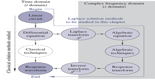
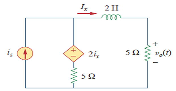
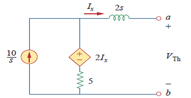
Circuit analysis with Laplace transforms

  • Transform the circuit from the time domain to the s-domain.

  • Solve the circuit using any circuit analysis technique

  • Take the inverse transform of the solution to convert in the time domain.

image
SECTION 01

Circuit Element Models

  • \[\begin{aligned} v(t) & = Ri(t) \\ V(s) & = RI(s) \end{aligned}\]
    Resistor
  • Inductor

    \[\begin{aligned} v(t) & = L \dfrac{di(t)}{dt} \\ V(s) & = L[sI(s)-i(0^-)] = sLI(s)-Li(0^-)\\ I(s) & = \dfrac{1}{sL}V(s)+\dfrac{i(0^-)}{s} \end{aligned}\]
  • Capacitor

    \[\begin{aligned} i(t) & = C\dfrac{dv(t)}{dt} \\ I(s) & = C[sV(s)-v(0^-)] = sCV(s)-Cv(0^-)\\ V(s) & = \dfrac{1}{sC}I(s)+\dfrac{v(0^-)}{s} \end{aligned}\]
  • Assuming zero initial condition for L and C

\[\begin{array}{lll} {\color{magenta}{\textbf{ Resistor: }}} & V(s)=R I(s) & Z(s)=R \\ {\color{blue}{\textbf{Inductor: }}} & V(s)=s L I(s) & Z(s)=s L \\ {\color{red}{\textbf{Capacitor: }}} & V(s)=\dfrac{1}{s C} I(s) & Z(s)=\dfrac{1}{s C} \end{array}\]
  • LT in circuit analysis facilitates the use of various signal sources such as impulse, step, ramp, exponential, and sinusoidal.

SECTION 01

Problem

  • Find \(v_0(t)\) assuming zero initial conditions.

image
\[\begin{aligned} u(t) & \Rightarrow \frac{1}{s} \quad 1 \mathrm{H} \Rightarrow \quad s L=s \\ \frac{1}{3} \mathrm{~F} \quad & \Rightarrow \quad \frac{1}{s C}=\frac{3}{s} \\ \end{aligned}\]
\[\begin{aligned} {\color{magenta}{\textbf{Mesh-1}}}~~\frac{1}{s} &=\left(1+\frac{3}{s}\right) I_{1}-\frac{3}{s} I_{2} \\ {\color{magenta}{\textbf{Mesh-2}}}~~0 &=-\frac{3}{s} I_{1}+\left(s+5+\frac{3}{s}\right) I_{2} \\ V_{o}(s) &=s I_{2}=\frac{3}{s^{2}+8 s+18}=\frac{3}{\sqrt{2}} \frac{\sqrt{2}}{(s+4)^{2}+(\sqrt{2})^{2}} \\ v_{o}(t) &=\frac{3}{\sqrt{2}} e^{-4 t} \sin \sqrt{2 t} \mathrm{~V}, \quad t \geq 0 \end{aligned}\]
SECTION 01

Problem

  • Find \(v_0(t)\) assuming \(v_0(0)=5\) V

image
\[\begin{aligned} & Cv_0 = 0.5~\mathrm{A}~\text{Initial current} \\ & {\color{magenta}{\textbf{Nodal analysis}}} \\ &\frac{10 /(s+1)-V_{o}}{10}+2+0.5=\frac{V_{o}}{10}+\frac{V_{o}}{10 / s} \\ &V_{o}=\frac{25 s+35}{(s+1)(s+2)}=\frac{A}{s+1}+\frac{B}{s+2} \end{aligned}\]
\[\begin{aligned} &A=\left.(s+1) V_{o}(s)\right|_{s=-1}=\left.\frac{25 s+35}{(s+2)}\right|_{s=-1}=\frac{10}{1}=10 \\ &B=\left.(s+2) V_{o}(s)\right|_{s=-2}=\left.\frac{25 s+35}{(s+1)}\right|_{s=-2}=\frac{-15}{-1}=15 \\ &V_{o}(s)=\frac{10}{s+1}+\frac{15}{s+2} \quad \Rightarrow ~~ v_{o}(t)=\left(10 e^{-t}+15 e^{-2 t}\right) u(t) \mathrm{V} \end{aligned}\]
SECTION 01

Problem

  • \[\begin{aligned} v_s(t)&=10u(t) ~\mathrm{V}\\ i_L(0)&=-1~\mathrm{A} \\ v_c(0)&=5 ~\mathrm{V} \end{aligned}\]
    assuming Find
image
\[\begin{aligned} &\frac{V_{1}-10 / s}{10 / 3}+\frac{V_{1}-0}{5 s}+\frac{i(0)}{s}+\frac{V_{1}-[v(0) / s]}{1 /(0.1 s)}=0 \\ &0.1\left(s+3+\frac{2}{s}\right) V_{1}=\frac{3}{s}+\frac{1}{s}+0.5 \\ &V_{1}=\frac{40+5 s}{(s+1)(s+2)}=\frac{35}{s+1}-\frac{30}{s+2} \qquad \Rightarrow ~ v_{1}(t)=\left(35 e^{-t}-30 e^{-2 t}\right) u(t) \mathrm{V} \end{aligned}\]
SECTION 01

Problem

  • Find \(V_0(s)\) using Thevenin’s theorem assuming no intial energy stored at \(t=0\) and \(i_s=10u(t)\) A.

image
image
\[V_{oc} = V_{Th} = 5\left(\dfrac{10}{s}\right) = \dfrac{50}{s}\]
\[\begin{aligned} &I_{x}=\frac{V_{1}}{2 s} \\ &-\frac{10}{s}+\frac{\left(V_{1}-2 I_{x}\right)-0}{5}+\frac{V_{1}-0}{2 s}=0 \\ &V_{1}=\frac{100}{2 s+3} \\ &I_{\mathrm{sc}}=\frac{V_{1}}{2 s}=\frac{100 /(2 s+3)}{2 s}=\frac{50}{s(2 s+3)} \\ &Z_{\mathrm{Th}}=\frac{V_{\mathrm{oc}}}{I_{\mathrm{sc}}}=\frac{50 / s}{50 /[s(2 s+3)]}=2 s+3 \end{aligned}\]
\[\begin{aligned} V_{o}&=\frac{5}{5+Z_{\mathrm{Th}}} V_{\mathrm{Th}}\\ &=\frac{5}{5+2 s+3}\left(\frac{50}{s}\right)\\ &=\frac{250}{s(2 s+8)}=\frac{125}{s(s+4)} \end{aligned}\]