Phase-Controlled DC Drives – Operating Modes | Solid-State Drives

SECTION 01

1. Operating Modes of DC Drives

Introduction to Operating Modes

In variable-speed applications, a DC motor operates in different modes:

Motoring
Normal driving operation
Regenerative Braking
Energy recovery to supply
Dynamic Braking
Energy dissipation in resistor

Plugging
Reverse voltage braking
Four-Quadrant Operation
Forward/reverse motoring and braking

Implementation

Different modes require switching power semiconductor devices and contactors to reconfigure field and armature circuits.

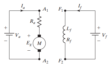
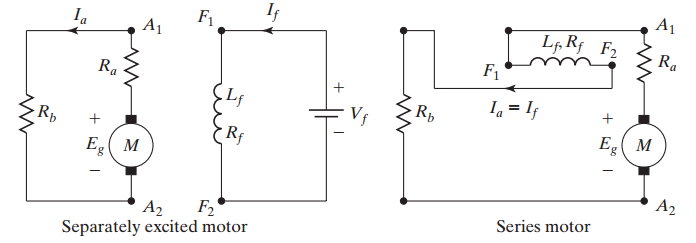
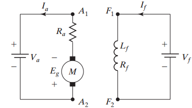
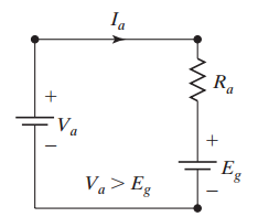
1.1 Motoring Mode

Motoring Mode – Separately Excited Motor

Characteristics:

Back EMF: \(E_g < V_a\) (supply voltage)
Both \(I_a > 0\) and \(I_f > 0\)
Motor develops torque to meet load demand
Energy flows from supply to motor
Normal driving operation

Governing Equations:

\[ \begin{aligned} V_a &= E_g + I_a R_a \\ E_g &= K_v \omega I_f \\ T_d &= K_t I_f I_a \end{aligned} \]

Condition: \(V_a > E_g\), \(I_a, I_f > 0\)

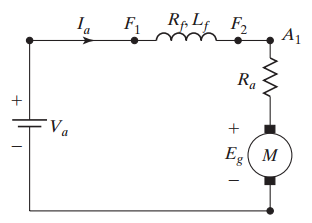
Circuit diagram of separately excited DC motor in motoring mode showing armature and field connections — Fig. 1 – Separately excited motor in motoring mode

Motoring Mode – Series Motor

Characteristics:

Series connection: \(I_a = I_f\)
High starting torque capability
Torque proportional to current squared
Voltage distributed across total resistance

Governing Equations:

\[ \begin{aligned} V_a &= E_g + I_a(R_a + R_f) \\ T_d &= K_t I_a^2 \\ I_a &= I_f \end{aligned} \]

Advantage: Excellent for traction applications requiring high starting torque.

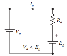
Circuit diagram of series DC motor in motoring mode — Fig. 2 – Series motor in motoring mode

1.2 Regenerative Braking

Regenerative Braking – Concept

What is Regenerative Braking?

Operating Principle:

Motor acts as a generator
Kinetic energy → electrical energy
Energy returned to the supply
Reduces overall energy consumption
Environmentally friendly and cost-effective

Applications:

Electric vehicles
Elevators and cranes
Railway traction systems
Industrial drives with frequent stops

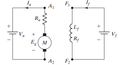
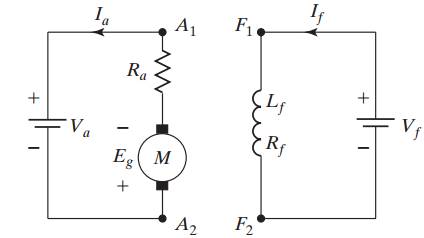
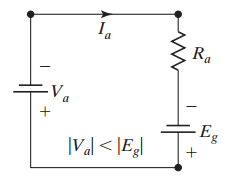
Conditions for Regenerative Braking

Back EMF exceeds supply: \(E_g > V_a\)
Armature current reverses: \(I_a < 0\)
Field current remains positive: \(I_f > 0\)
Supply must be receptive (able to accept power)

Regenerative Braking – Separately Excited Motor

Operating Principle:

Motor rotates due to inertia or load
Generated EMF exceeds supply voltage
Current flows back to supply
Braking torque opposes motion
Speed decreases gradually

Governing Equations:

\[ \begin{aligned} E_g &> V_a \\ I_a &= \frac{E_g - V_a}{R_a} < 0 \\ P_{\text{regen}} &= (E_g - V_a)|I_a| \end{aligned} \]

Energy Flow: Motor → Supply

Circuit diagram showing regenerative braking in separately excited DC motor — Fig. 3 – Regenerative braking in separately excited motor

Regenerative Braking – Series Motor

Special Requirements:

Motor must operate as self-excited generator
Field current must aid residual flux
Reverse either armature or field terminals (not both)
Requires careful control to maintain excitation

Critical Condition

For self-excitation to occur, the field current direction must reinforce residual magnetism in the field winding.

Challenge: Maintaining stable voltage buildup during braking.

Circuit diagram showing series motor connection for regenerative braking — Fig. 4 – Series motor connection for regenerative braking

1.3 Dynamic Braking

Dynamic Braking – Concept

What is Dynamic Braking?

Operating Principle:

Armature disconnected from supply
Armature connected to braking resistor
Kinetic energy dissipated as heat
No energy returned to supply
Independent of supply availability

Advantages:

Simple implementation
No receptive supply required
Smooth, controlled braking
Effective at high speeds

Disadvantages:

Energy wasted as heat
Requires heat dissipation capacity
Less efficient than regenerative braking

Key Condition

Field excitation must be maintained during braking operation.

Dynamic Braking – Separately Excited Motor

Operating Principle:

Armature disconnected from supply
Armature terminals connected to resistor \(R_B\)
Field excitation maintained separately
Generated EMF drives current through resistor
Braking torque proportional to speed

Governing Equations:

\[ \begin{aligned} E_g &= I_a(R_a + R_B) \\ I_a &= \frac{K_v \omega I_f}{R_a + R_B} \\ T_B &= K_t I_f I_a \\ P_{\text{dissipated}} &= I_a^2(R_a + R_B) \end{aligned} \]

Circuit diagram of dynamic braking in separately excited DC motor with braking resistor — Fig. 5 – Dynamic braking in separately excited motor

Dynamic Braking – Series Motor

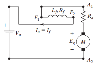
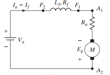
Special Configuration:

Armature and field must be reconnected
Field can be connected in series or parallel with armature
Both connected across braking resistor
Ensures field excitation is maintained

Governing Equations – Series Configuration:

\[ \begin{aligned} E_g &= I_a(R_a + R_f + R_B)\\ I_a &= I_f \end{aligned} \]

Note: Field-armature reconfiguration ensures adequate excitation during braking.

Circuit diagram of series DC motor in dynamic braking mode — Fig. 6 – Series motor in dynamic braking mode

1.4 Plugging

Plugging – Concept

What is Plugging?

A reverse voltage braking method
Supply polarity is reversed while the motor is still running
Both \(V_a\) and back-EMF \(E_g\) oppose armature current in the same direction
Produces the largest braking torque among all electrical braking methods

Operating Principle:

Reversed \(V_a\) and \(E_g\) act additively against current flow
Results in very high armature current
A current-limiting resistor \(R_p\) is inserted in series
Motor must be disconnected as speed approaches zero

Critical Warning

If not disconnected at zero speed, the motor will accelerate in the reverse direction .

Plugging – Circuit Configuration

Circuit diagram of plugging in a separately excited DC motor — Fig. 7 – Plugging in separately excited DC motor

Circuit diagram of plugging in a series excited DC motor — Fig. 8 – Plugging in series excited DC motor

Governing Equations:

\[ \begin{aligned} I_a &= \frac{V_a + E_g}{R_a + R_f} \\ T_B &= K_t\,I_f\,I_a \\ P_{\text{loss}} &= (V_a + E_g)\,I_a \end{aligned} \]

Plugging – Characteristics, Applications & Limitations

Characteristics:

Fastest braking action among all methods
Very high armature current during braking
Significant energy dissipated in \(R_p\)
Considerable mechanical stress on the motor shaft

Applications:

Emergency stops
Rapid direction reversals
Elevators and hoists
Machine tools requiring quick halts

Limitations:

Very low energy efficiency
High thermal stress on resistor and windings
Requires robust current-limiting circuitry
Needs automatic disconnection sensing at \(\omega = 0\)

Comparison Note

Plugging offers the fastest stop but at the cost of highest energy loss and maximum mechanical stress compared to dynamic or regenerative braking.

1.5 Comparison of Braking Methods

Comparison of Braking Methods

Comprehensive comparison of braking methods
Parameter	Regenerative	Dynamic	Plugging
Energy Recovery	Yes	No	No
Braking Speed	Moderate	Moderate	Very Fast
Supply Required	Yes (receptive)	No	Yes
Energy Efficiency	High	Low	Very Low
Circuit Complexity	High	Low	Moderate
Current Magnitude	Normal	Normal	Very High
Typical Applications	Frequent stops	Emergency	Quick reversal
Initial Cost	High	Low	Moderate
Operating Cost	Low	Moderate	High

Selection Criteria

Choose based on: energy recovery needs, braking frequency, supply receptivity, and cost constraints.

SECTION 02

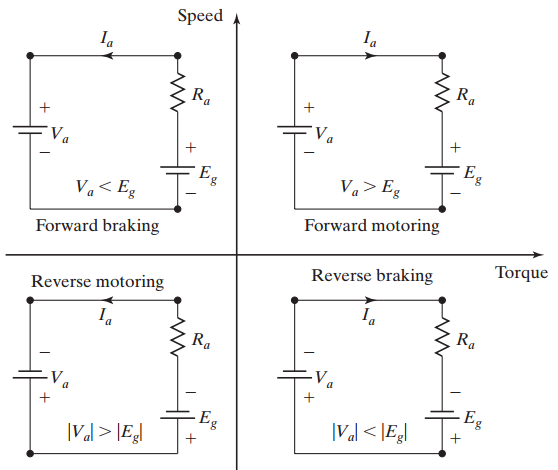
2. Four-Quadrant Operation

Four-Quadrant Operation – Overview

Quadrants Defined By:

Torque direction: positive/negative
Speed direction: positive/negative

Power Flow:

Motoring (Q-I, Q-III): Supply → Motor
Braking (Q-II, Q-IV): Motor → Supply

Applications:

Elevators and lifts
Rolling mills
Machine tools
Electric vehicles

Four-quadrant operation torque-speed diagram showing all four operating regions — Fig. 9 – Four-quadrant operation diagram

Quadrant I – Forward Motoring

Characteristics:

Speed: Positive (\(\omega > 0\))
Torque: Positive (\(T_d > 0\))
\(V_a > 0\), \(E_g > 0\), \(I_a > 0\)
Normal forward driving
Power flows from supply to motor

Governing Conditions:

\[ \begin{aligned} V_a &> E_g \\ V_a &> 0, \quad I_a &> 0 \\ E_g &= K_v \omega I_f &> 0 \\ T_d &= K_t I_f I_a &> 0 \end{aligned}\]

Circuit and quadrant diagram for forward motoring – Quadrant I — Fig. 10 – Forward motoring (Quadrant I)

Energy Flow

Supply → ^Power → Motor → ^Torque → Load

Quadrant II – Forward Regenerative Braking

Characteristics:

Speed: Positive (\(\omega > 0\))
Torque: Negative (\(T_d < 0\))
\(V_a > 0\), \(E_g > 0\), \(I_a < 0\)
Forward regenerative braking
Power flows from motor to supply

Governing Conditions:

\[ \begin{aligned} E_g &> V_a \\ V_a &> 0, \quad I_a & < 0 \\ |E_g| &> |V_a| \\ T_d &= K_t I_f I_a & < 0 \end{aligned} \]

Circuit and quadrant diagram for forward regenerative braking – Quadrant II — Fig. 11 – Forward regenerative braking (Quadrant II)

Energy Flow

Load → ^KE → Motor → ^Power → Supply

Quadrant III – Reverse Motoring

Characteristics:

Speed: Negative (\(\omega < 0\))
Torque: Negative (\(T_d < 0\))
\(V_a < 0\), \(E_g < 0\), \(I_a < 0\)
Normal reverse driving
Power flows from supply to motor

Governing Conditions:

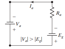
\[ \begin{aligned} |V_a| &> |E_g| \\ V_a & < 0, \quad I_a &< 0 \\ E_g &=K _v \omega I_f &< 0 \\ T_d &=K _t I_f I_a &< 0 \end{aligned} \]

Circuit and quadrant diagram for reverse motoring – Quadrant III — Fig. 12 – Reverse motoring (Quadrant III)

Implementation

Reverse field excitation to reverse \(E_g\) polarity, or reverse armature terminals.

Quadrant IV – Reverse Regenerative Braking

Characteristics:

Speed: Negative (\(\omega < 0\))
Torque: Positive (\(T_d > 0\))
\(V_a < 0\), \(E_g < 0\), \(I_a > 0\)
Reverse regenerative braking
Power flows from motor to supply

Governing Conditions:

\[ \begin{aligned} |E_g| &> |V_a| \\ V_a &< 0, \quad I_a > 0 \\ E_g &< 0, \quad \omega < 0 \\ T_d &= K_t I_f I_a > 0 \end{aligned}\]

Circuit and quadrant diagram for reverse regenerative braking – Quadrant IV — Fig. 13 – Reverse regenerative braking (Quadrant IV)

Energy Flow

Load → ^KE → Motor → ^Power → Supply

Summary of Four-Quadrant Operation

Comprehensive summary of four-quadrant operation
Parameter	Q-I	Q-II	Q-III	Q-IV
Operation	Fwd Motoring	Fwd Braking	Rev Motoring	Rev Braking
Speed \(\omega\)	+	+	−	−
Torque \(T_d\)	+	−	−	+
Voltage \(V_a\)	+	+	−	−
EMF \(E_g\)	+	+	−	−
Current \(I_a\)	+	−	−	+
Voltage Relation	\(V_a > E_g\)	\(E_g > V_a\)	\(\|V_a\| > \|E_g\|\)	\(\|E_g\| > \|V_a\|\)
Power Flow	Supply→Motor	Motor→Supply	Supply→Motor	Motor→Supply
Mode Type	Motoring	Regenerative	Motoring	Regenerative

Key Requirement for Q-III and Q-IV

Field excitation or armature polarity must be reversed for operations in Quadrants III and IV.

SECTION 03

3. Key Takeaways

Key Takeaways

Operating Modes:
- DC motors support multiple operating modes: motoring, regenerative braking, dynamic braking, and plugging.
- Each mode has distinct voltage-current relationships and energy flow patterns.
Energy Efficiency:
- Regenerative braking offers highest efficiency by returning energy to supply.
- Dynamic braking provides supply-independent operation at cost of efficiency.
- Plugging provides fastest braking but with highest losses.
Four-Quadrant Operation:
- Enables complete bidirectional control (forward/reverse motoring and braking).
- Critical for applications requiring frequent direction reversals.
- Requires appropriate power electronic converters and control schemes.