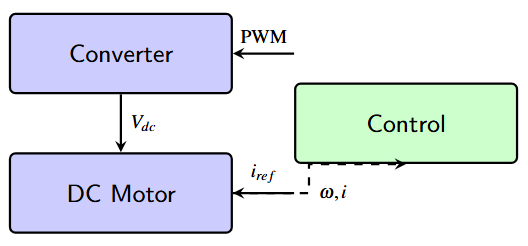
Introduction to DC Drives
A DC drive is a system that controls the speed, torque, and direction of a DC motor through power electronic converters.
Main Components:
- DC motor (separately excited or series)
- Power electronic converter
- Control circuit
Provides variable speed operation through voltage/current control.
Key Feature
Ability to provide continuously variable DC voltage from fixed AC or DC source
Industrial Applications:
- Rolling mills
- Paper machines
- Textile mills
- Machine tools
- Cranes and hoists
- Elevators
Transportation:
- Electric traction (trains, trams)
- Battery electric vehicles
- Mass rapid transit systems
- Mining equipment
Power Range
From fractional horsepower to several megawatts
- Variable speed control: Wide range and smooth operation
- High starting torque: Excellent for heavy loads
- Simple control: Relatively simpler than AC drives
- Good dynamic response: Fast acceleration/deceleration
- Four-quadrant operation: Forward/reverse motoring and braking
- Regenerative braking: Energy recovery capability
- Precise speed regulation: Excellent for positioning applications
Motor Limitations:
- Commutator and brushes require maintenance
- Not suitable for very high speeds
- Higher cost than AC motors
- Limited to lower speeds
Drive System Issues:
- Supply harmonics
- Acoustic noise
- Motor derating
- Space and cooling requirements
- Capital cost
- EMI/EMC issues (PWM drives)
Future Trend
AC drives are becoming increasingly competitive, but DC drives will remain relevant for several more decades
Based on Input Power Supply:
-
Single-Phase Drives
- Power range: up to 100 kW
- Applications: Small to medium power
-
Three-Phase Drives
- Power range: 100 kW to 1500 kW
- Applications: Medium to high power
- Can be connected in series/parallel for 12-pulse output
-
DC-DC Converter Drives (Chopper Drives)
- Fed from DC source (battery or rectified DC)
- Applications: Traction, electric vehicles, MRT systems
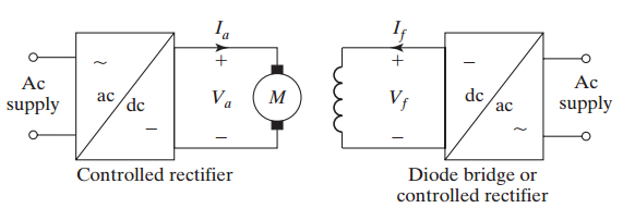
Configuration 1: Controlled Rectifier-Fed Drive
AC supply \(\rightarrow\) Controlled Rectifier \(\rightarrow\) DC Motor
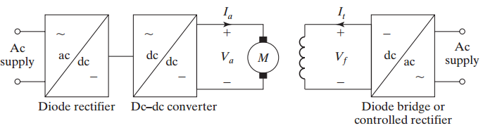
Configuration 2: DC-DC Converter-Fed Drive
AC supply \(\rightarrow\) Diode Rectifier \(\rightarrow\) DC-DC Converter \(\rightarrow\) DC Motor
Note
Both configurations can control armature and field circuits independently
Basic Characteristics of DC Motors
Based on Field Winding Connection:
-
Separately Excited DC Motor
- Field excitation independent of armature circuit
- Also called shunt-field motor
- Armature and field currents are different
- Field current \(I_f\) is much less than armature current \(I_a\)
-
Series Excited DC Motor
- Field winding connected in series with armature
- Armature and field currents are the same (\(I_a = I_f\))
- High starting torque
- Commonly used in traction applications
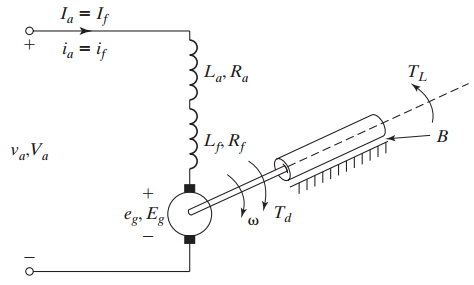
Separately Excited DC Motor
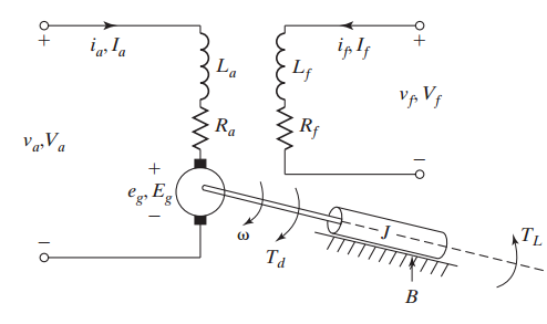
Circuit Parameters:
- \(V_a\): Applied armature voltage
- \(R_a\): Armature resistance
- \(L_a\): Armature inductance
- \(E_b\): Back EMF
- \(I_a\): Armature current
- \(V_f\): Field voltage
- \(I_f\): Field current
Voltage Equation
In steady state (\(\frac{dI_a}{dt} = 0\)):
Back EMF
where:
- \(K_a\): Armature constant
- \(\phi\): Field flux
- \(\omega_m\): Mechanical angular velocity (rad/s)
Electromagnetic Torque
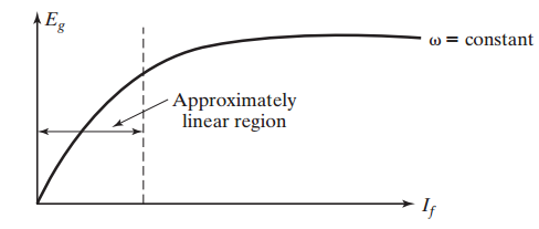
Field Flux
where \(K_f\) is the field constant (in the linear region)
From the steady-state voltage equation:
Solving for speed:
Since \(T_e = K_a \phi I_a\), we have \(I_a = \frac{T_e}{K_a \phi}\)
Speed-Torque Relationship
This is a linear relationship with negative slope
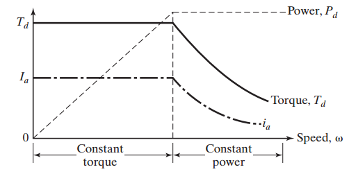
1. Armature Voltage Control
- Keep field current \(I_f\) constant (constant flux)
- Vary armature voltage \(V_a\)
- Speed is proportional to \(V_a\)
- Used for speeds below base speed
- Constant torque region
2. Field Current Control (Field Weakening)
- Keep armature voltage at rated value
- Reduce field current \(I_f\) (weaken flux)
- Speed increases as flux decreases
- Used for speeds above base speed
- Constant power region
Important Note
Field weakening allows speed increase but reduces available torque. Maximum torque decreases as \(1/\omega_m\), keeping power constant.
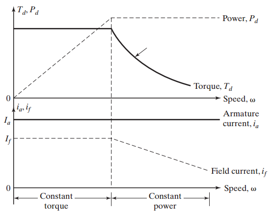
Region I: Constant Torque
- Speed range: 0 to base speed
- Method: Armature voltage control
- \(\phi = \text{constant}\)
- \(T_{max} = \text{constant}\)
- \(P \propto \omega_m\)
Region II: Constant Power
- Speed range: Base speed to maximum
- Method: Field weakening
- \(\phi \propto 1/\omega_m\)
- \(T_{max} \propto 1/\omega_m\)
- \(P = \text{constant}\)
Input Power:
Armature Copper Loss:
Field Copper Loss:
Developed Power:
Output Mechanical Power:
where \(P_{rot}\) includes friction, windage, and core losses
Efficiency
Series Excited DC Motor
Key Characteristic:
In a series motor, the field winding is connected in series with the armature, therefore:
Voltage Equation
where \(R_f\) is the field winding resistance
Back EMF
Torque
Important: Torque is proportional to the square of current!
From the voltage equation:
Since \(T_e = K_a K_f I^2\), we have \(I = \sqrt{\frac{T_e}{K_a K_f}}\)
Substituting and solving for speed:
Critical Characteristic
Speed varies inversely with the square root of torque: \(\omega_m \propto 1/\sqrt{T_e}\)
Danger: At no load (low torque), speed can become dangerously high!
Advantages
- Very high starting torque
- Good for variable loads
- Automatic speed adjustment
- Simple construction
Disadvantages
- Dangerous at no load
- Poor speed regulation
- Limited speed control range
- Not suitable for constant speed
Typical Applications:
- Electric traction (trains, metros)
- Cranes and hoists
- Conveyor belts
- Electric vehicles
- Any application requiring high starting torque
| Parameter | Separately Excited | Series |
|---|---|---|
| Connection | Field independent | Field in series |
| Current Relation | \(I_a \neq I_f\) | \(I_a = I_f\) |
| Starting Torque | High | Very High |
| Speed Regulation | Good | Poor |
| No-Load Speed | Finite | Very high (dangerous) |
| Control Complexity | Moderate | Simple |
| Main Application | Industrial drives | Traction |
| Speed Range | Wide | Limited |
| Torque vs Current | Linear (\(T \propto I_a\)) | Quadratic (\(T \propto I_a^2\)) |
Gear Ratio Analysis
Why use a gearbox?
- Motors designed for high speeds (smaller size, lower cost)
- Most applications require lower speeds
- Gearbox acts as a torque transformer
- Amplifies torque at load side while reducing speed
Design Principle
Higher speed \(\implies\) Lower volume and size of motor for same power
For constant power, higher speed means lower torque requirement
Trade-off
Gearbox adds cost, size, and losses, but enables optimal motor design
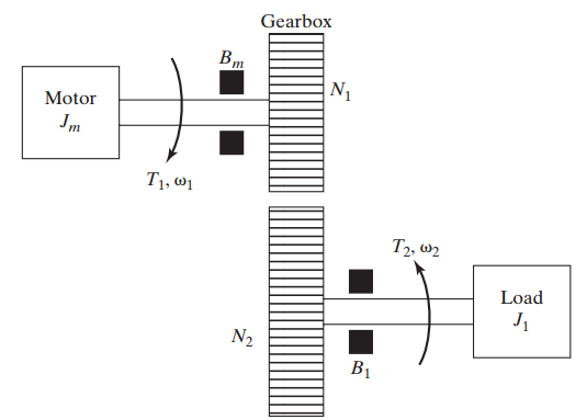
System Components:
- Motor side: \(J_m\), \(B_m\), \(T_1\), \(\omega_1\), \(N_1\)
- Load side: \(J_L\), \(B_L\), \(T_2\), \(\omega_2\), \(N_2\)
where:
- \(J\): Moment of inertia
- \(B\): Friction coefficient
- \(T\): Torque
- \(\omega\): Angular velocity
- \(N\): Number of gear teeth
Power Conservation (Lossless Gearbox)
Speed Ratio
Torque Transformation
Gear Ratio
To simplify analysis, load parameters can be reflected to the motor side:
Reflected Load Inertia
Reflected Friction Coefficient
Equivalent Motor Torque
High Gear Ratio (\(GR \gg 1\)):
- Large speed reduction
- Large torque amplification at load
- Load inertia and friction have minimal effect on motor
- Motor sees very small reflected load
Low Gear Ratio (\(GR \approx 1\)):
- Minimal speed reduction
- Minimal torque amplification
- Load inertia and friction significantly affect motor
Design Consideration
Proper gear ratio selection is crucial for optimal system performance
Example
For \(GR = 10\): Reflected load inertia = \(\dfrac{J_L}{100}\)
Gearbox Characteristics:
- Real gearboxes have losses (typically 2–5% per stage)
- Backlash can affect positioning accuracy
- Additional inertia of gears must be considered
- Maintenance requirements
- Cost and size
Applications Without Gearbox:
- Direct drive systems (high-torque motors)
- Applications requiring high positioning accuracy
- High-speed applications (spindles, fans)
Summary
- DC Drives provide variable speed control for DC motors using power electronic converters
- Three types based on supply: Single-phase, Three-phase, and DC-DC converter drives
-
Two main motor types:
- Separately excited: Industrial applications
- Series: Traction applications (high starting torque)
-
Speed control methods:
- Armature voltage control (below base speed)
- Field current control (above base speed)
-
Operating regions:
- Constant torque: 0 to base speed (armature control)
- Constant power: above base speed (field weakening)
- Gearbox: Acts as torque transformer, enables optimal motor design, load parameters reflected by \(1/GR^2\)
- Future trend: AC drives becoming competitive, but DC drives remain important