Recap from Lec-2A

Key equations derived:

EMF Equation

\[E = K_e\omega_m\]

Torque Equation

\[T_e = K_t I_a = K_e I_a\]

Today's focus:

How does armature circuit behave with resistance and inductance?
What about the field circuit?
How to model mechanical dynamics?
How to combine electrical and mechanical subsystems?

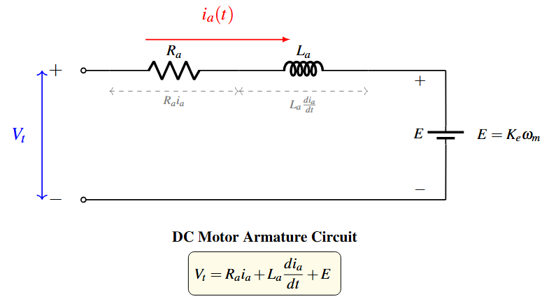
Armature Circuit Modeling

Armature Circuit Components

Physical components in armature circuit:

Resistance:

Copper winding resistance
Brush contact resistance
Combined as \(R_a\)
Causes power loss (\(I_a^2 R_a\))

Inductance:

Self-inductance of windings
Magnetic energy storage
Denoted as \(L_a\)
Affects transient response

Back-EMF:

Generated EMF \(E = K_e\omega_m\)
Opposes applied voltage (Lenz's law)
Speed-dependent voltage
Key coupling between electrical and mechanical systems

Armature Circuit Equivalent

Note

The back-EMF \(E\) acts like a voltage source that opposes the applied voltage \(V\). Its magnitude depends on the rotor speed \(\omega_m\).

Armature Circuit Equation

Applying Kirchhoff's Voltage Law (KVL) around armature circuit:

\[V = R_a I_a + L_a\frac{dI_a}{dt} + E\]

Substituting \(E = K_e\omega_m\):

Dynamic Armature Equation

\[\boxed{V = R_a I_a + L_a\frac{dI_a}{dt} + K_e\omega_m}\]

This is a first-order differential equation relating:

Applied voltage \(V\) (input)
Armature current \(I_a\) (electrical variable)
Rotor speed \(\omega_m\) (mechanical variable)

Steady-State Armature Equation

In steady state, all variables are constant:

\[\frac{dI_a}{dt} = 0\]

Steady-State Armature Equation

\[\boxed{V = R_a I_a + K_e\omega_m}\]

Solving for armature current:

\[I_a = \frac{V - K_e\omega_m}{R_a} = \frac{V - E}{R_a}\]

Observations:

As speed increases, back-EMF increases
Higher back-EMF reduces armature current
At no load, \(I_a\) is small, \(E \approx V\)

Armature Circuit Time Constant

Rearranging the dynamic equation:

\[L_a\frac{dI_a}{dt} = V - R_a I_a - K_e\omega_m\]

\[\frac{dI_a}{dt} = -\frac{R_a}{L_a}I_a - \frac{K_e}{L_a}\omega_m + \frac{1}{L_a}V\]

Electrical Time Constant

\[\boxed{\tau_a = \frac{L_a}{R_a} \text{ seconds}}\]

Physical significance:

Determines how fast armature current responds to voltage changes
Typical values: 5–50 ms (milliseconds)
Smaller \(\tau_a\) \(\rightarrow\) faster electrical response
After time \(\tau_a\), current reaches approximately 63% of its final value

Power Flow in Armature Circuit

Multiplying armature equation by \(I_a\):

\[VI_a = R_a I_a^2 + L_a I_a\frac{dI_a}{dt} + K_e\omega_m I_a\]

Power Balance

\[\underbrace{VI_a}_{\substack{\text{Electrical}\\\text{Input Power}}} = \underbrace{R_a I_a^2}_{\substack{\text{Armature}\\\text{Copper Loss}}} + \underbrace{L_a I_a\frac{dI_a}{dt}}_{\substack{\text{Stored in}\\\text{Inductance}}} + \underbrace{K_e\omega_m I_a}_{\substack{\text{Converted to}\\\text{Mechanical}}}\]

In steady state: \(\dfrac{dI_a}{dt} = 0\)

\[\boxed{VI_a = R_a I_a^2 + K_e\omega_m I_a = R_a I_a^2 + EI_a}\]

\(EI_a\) = Air gap power = Electromagnetic power developed
\(R_a I_a^2\) = Copper loss (heat dissipated)

Field Circuit Modeling

Field Circuit for Separately Excited Motor

Separately Excited DC Motor:

Field and armature circuits are independent
Field supplied from separate DC source
Allows independent control of flux and torque

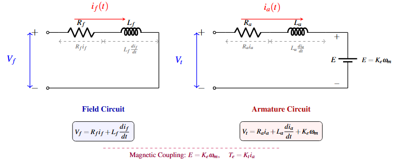
Separately Excited Motor circuit diagram and equations — Separately Excited Motor Equations

Field Circuit Equation

Applying KVL to field circuit:

\[V_f = R_f I_f + L_f\frac{dI_f}{dt}\]

Where:

\(V_f\) = Field supply voltage (DC)
\(R_f\) = Field winding resistance (typically large)
\(L_f\) = Field winding inductance (very large)
\(I_f\) = Field current

Field Time Constant

\[\boxed{\tau_f = \frac{L_f}{R_f} \text{ seconds}}\]

Typical values: 0.5 to 2 seconds

Key observation: Field circuit is much slower than armature circuit (\(\tau_f \gg \tau_a\))

Flux-Current Relationship

For unsaturated magnetic circuit:

\[\phi = L_{af} I_f\]

Where:

\(\phi\) = Air-gap flux per pole (Wb)
\(L_{af}\) = Mutual inductance between armature and field
\(I_f\) = Field current (A)

Torque constant relationship:

\[K_e = K_t = k\phi = kL_{af}I_f\]

For constant field current, \(K_e\) and \(K_t\) are constants.

Simplified Field Model

For many control applications:

Field current is kept constant by a controlled supply
Field dynamics are much slower than armature and mechanical dynamics
Assumption: \(I_f = \text{constant}\) during transients

Practical Note

In armature-controlled DC motors, field excitation is fixed, and motor speed/torque is controlled by varying armature voltage. This simplifies the analysis significantly.

Mechanical System Modeling

Mechanical System Components

Rotating mechanical system includes:

Inertia (J):

Rotor inertia
Load inertia (reflected to motor shaft)
Unit: kg·m²
Resists changes in speed

Friction (B):

Viscous friction (proportional to speed)
Bearing friction
Windage losses
Unit: N·m·s/rad

Load Torque (\(T_L\)):

External torque demand from the load
Can be constant, speed-dependent, or time-varying
Unit: N·m

Newton's Second Law for Rotation

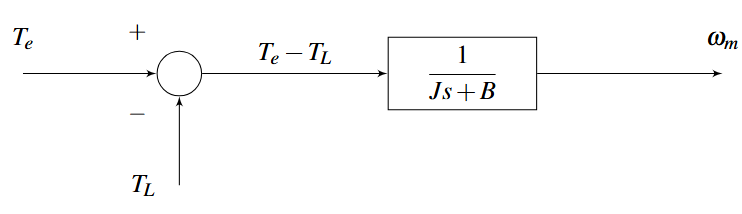
Applying Newton's law to rotating system:

\[J\frac{d\omega_m}{dt} = \text{Net Torque}\]

Net torque = Electromagnetic torque - Friction torque - Load torque:

Dynamic Mechanical Equation

\[\boxed{J\frac{d\omega_m}{dt} = T_e - B\omega_m - T_L}\]

Where:

\(T_e = K_e I_a\) = Electromagnetic torque developed by motor
\(B\omega_m\) = Friction torque (opposes motion)
\(T_L\) = Load torque (opposes motion)

Mechanical Time Constant

Rearranging the mechanical equation:

\[\frac{d\omega_m}{dt} = \frac{K_e}{J}I_a - \frac{B}{J}\omega_m - \frac{1}{J}T_L\]

Mechanical Time Constant

\[\boxed{\tau_m = \frac{J}{B} \text{ seconds}}\]

Physical significance:

Determines how fast the motor speed responds to torque changes
Typical values: 0.1 to 5 seconds
Slower than electrical time constant: \(\tau_m \gg \tau_a\)
After time \(\tau_m\), speed reaches approximately 63% of its final value

Steady-State Mechanical Equation

In steady state: \(\dfrac{d\omega_m}{dt} = 0\)

Steady-State Torque Balance

\[\boxed{T_e = B\omega_m + T_L}\]

Interpretation:

Electromagnetic torque must balance friction and load torque
At no-load (\(T_L = 0\)): \(T_e = B\omega_m\)
Higher load torque requires higher electromagnetic torque

Load Torque Characteristics

Types of Load Torque

Load torque can have different speed dependencies:

1. Constant Torque Load

\[T_L = T_0 = \text{constant}\]

Examples: Hoists, cranes, conveyor belts, friction loads

Torque independent of speed

2. Linear (Viscous) Load

\[T_L = k_1\omega_m\]

Examples: Generators with resistive load, some pumps

Torque proportional to speed

3. Quadratic (Fan-type) Load

\[T_L = k_2\omega_m^2\]

Examples: Fans, blowers, centrifugal pumps

Torque proportional to square of speed (fluid dynamics)

4. Constant Power Load

\[T_L = \frac{P_0}{\omega_m}\]

Examples: Machine tools, traction applications

Torque inversely proportional to speed

Impact on Motor Performance

Different load types affect motor behavior differently:

Constant torque: Motor must develop constant torque regardless of speed
Fan-type load: Light torque at low speed, increases rapidly at high speed
Constant power: High torque at low speed, decreases as speed increases

Design Consideration

Motor selection and drive design must account for the specific load torque characteristic to ensure adequate performance across the operating range.

Coupled Electromechanical Equations

Complete System Equations

For a separately excited DC motor with constant field current:

Electrical Subsystem

\[\boxed{V = R_a I_a + L_a\frac{dI_a}{dt} + K_e\omega_m}\]

Mechanical Subsystem

\[\boxed{J\frac{d\omega_m}{dt} = K_e I_a - B\omega_m - T_L}\]

Coupling Equations

\[\boxed{T_e = K_e I_a, \quad E = K_e\omega_m}\]

This is a coupled system of two first-order differential equations

State-Space Representation

Define state variables:

\(x_1 = I_a\) (armature current)
\(x_2 = \omega_m\) (rotor speed)

State equations:

State-Space Form

\[\begin{aligned} \frac{dx_1}{dt} = \frac{dI_a}{dt} &= -\frac{R_a}{L_a}I_a - \frac{K_e}{L_a}\omega_m + \frac{1}{L_a}V\\[0.3cm] \frac{dx_2}{dt} = \frac{d\omega_m}{dt} &= \frac{K_e}{J}I_a - \frac{B}{J}\omega_m - \frac{1}{J}T_L \end{aligned}\]

Input: \(V\) (control), \(T_L\) (disturbance)

Output: \(\omega_m\) (typically the variable of interest)

Matrix Form

In compact matrix notation:

\[\frac{d}{dt}\begin{bmatrix} I_a \\ \omega_m \end{bmatrix} = \begin{bmatrix} -\dfrac{R_a}{L_a} & -\dfrac{K_e}{L_a} \\[0.4cm] \dfrac{K_e}{J} & -\dfrac{B}{J} \end{bmatrix} \begin{bmatrix} I_a \\ \omega_m \end{bmatrix} + \begin{bmatrix} \dfrac{1}{L_a} & 0 \\[0.4cm] 0 & -\dfrac{1}{J} \end{bmatrix} \begin{bmatrix} V \\ T_L \end{bmatrix}\]

Standard form: \(\dot{\mathbf{x}} = \mathbf{A}\mathbf{x} + \mathbf{B}\mathbf{u}\)

where:

\(\mathbf{x} = [I_a \quad \omega_m]^T\) = state vector (2\(\times\)1)
\(\mathbf{u} = [V \quad T_L]^T\) = input vector (2\(\times\)1)
\(\mathbf{A}\) = system matrix (2\(\times\)2)
\(\mathbf{B}\) = input matrix (2\(\times\)2)

Block Diagram Representation

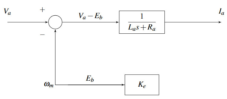
Block Diagram: Electrical Subsystem

Electrical block subsystem diagram showing transfer function from voltage to current — Electrical block subsystem

Transfer function from \((V - E)\) to \(I_a\):

\[\frac{I_a(s)}{V(s) - E(s)} = \frac{1}{R_a + L_a s} = \frac{1/R_a}{1 + \tau_a s}\]

Block Diagram: Mechanical Subsystem

Transfer function:

\[\frac{\omega_m(s)}{T_e(s) - T_L(s)} = \frac{1}{Js + B} = \frac{1/B}{1 + \tau_m s}\]

Complete Block Diagram

Transfer Function: Voltage to Speed

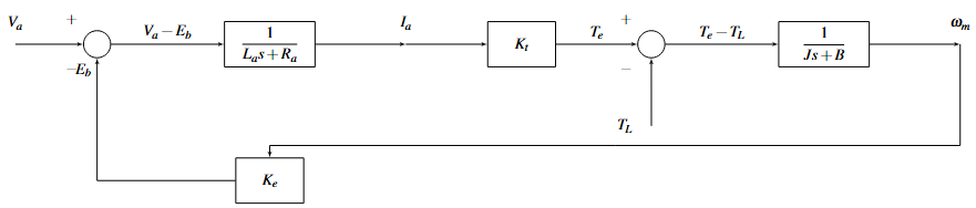
For no-load condition (\(T_L = 0\)):

Using block diagram algebra:

\[\frac{\omega_m(s)}{V(s)} = \frac{\dfrac{K_t}{(R_a + L_a s)(Js + B)}}{1 + \dfrac{K_e K_t}{(R_a + L_a s)(Js + B)}}\]

Simplifying:

Speed Transfer Function

\[\boxed{\frac{\omega_m(s)}{V(s)} = \frac{K_t}{(R_a + L_a s)(Js + B) + K_e K_t}}\]

This is a second-order system with both electrical and mechanical dynamics.

Simplified Model: Neglecting Armature Inductance

If \(L_a\) is very small, we can assume: \(L_a \approx 0\)

Transfer function becomes:

\[\frac{\omega_m(s)}{V(s)} = \frac{K_t}{R_a(Js + B) + K_e K_t} = \frac{K_t}{R_a Js + (R_a B + K_e K_t)}\]

First-Order Approximation

\[\boxed{\frac{\omega_m(s)}{V(s)} = \frac{K_t/(R_a B + K_e K_t)}{1 + \dfrac{R_a J}{R_a B + K_e K_t}s}}\]

DC gain: \(\dfrac{K_t}{R_a B + K_e K_t}\)

Time constant: \(\tau = \dfrac{R_a J}{R_a B + K_e K_t}\)

Summary and Key Takeaways

Summary: Circuit Equations

Armature Circuit (Dynamic)

\[V = R_a I_a + L_a\frac{dI_a}{dt} + K_e\omega_m\]

Time constant: \(\tau_a = L_a/R_a\) (5–50 ms)

Field Circuit (Dynamic)

\[V_f = R_f I_f + L_f\frac{dI_f}{dt}\]

Time constant: \(\tau_f = L_f/R_f\) (0.5–2 s)

Mechanical System (Dynamic)

\[J\frac{d\omega_m}{dt} = T_e - B\omega_m - T_L\]

Time constant: \(\tau_m = J/B\) (0.1–5 s)

Summary: Coupling and Hierarchy

Coupling equations:

\[T_e = K_e I_a, \quad E = K_e\omega_m\]

Time constant hierarchy:

\[\tau_a \ll \tau_m \ll \tau_f\]

Armature response is fastest (electrical)
Mechanical response is intermediate
Field response is slowest

Control implications:

Armature voltage control gives fast torque/speed control
Field control is slower but affects flux and torque capability
In transient analysis, field current often assumed constant

Key Concepts Covered

Armature circuit modeling
- \(R_a\), \(L_a\), and back-EMF
- Dynamic and steady-state equations
Field circuit modeling
- Separate excitation
- Much slower dynamics than armature
Mechanical system modeling
- Inertia, friction, and load torque
- Newton's law for rotation
Electromechanical coupling
- Two-way interaction through \(K_e\)
- State-space and block diagram representation
Load characteristics
- Different types: constant, linear, quadratic, constant power