Closed-Loop Control of DC Motors
A comprehensive three-part treatment: Foundations · System Design · Modern Control
Foundations & Separately Excited DC Motor Control
1. Why Closed-Loop Control?
Problem with Open-Loop Operation
- Speed changes if the firing angle is held constant while load torque increases.
- Maintaining constant speed requires continuous adjustment of the firing angle.
- Open-loop drives cannot do this automatically.
- Greater accuracy
- Improved dynamic response
- Reduced effect of load disturbances
- Enables rapid acceleration/deceleration
- Drive characteristics easily modified
- Built-in circuit protection
"Most industrial drive systems operate as closed-loop feedback systems."
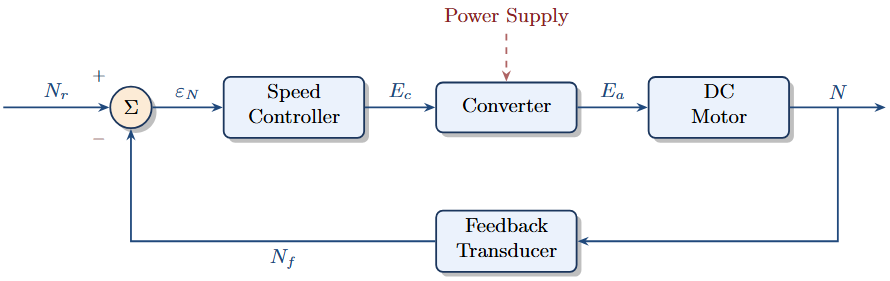
Basic Closed-Loop Speed-Control System
2. Separately Excited DC Motor — Overview
Key Features
- Separate excitation makes speed control relatively easy.
- Armature voltage is controlled in a closed-loop feedback system.
- Other protective features such as current limiting are incorporated.
Analysis Goal
- Derive transfer functions of the motor and control components.
- Assess the dynamic response of the drive.
Voltage loop:
Back-EMF:
Torque balance:
Developed torque:
3. Motor Transfer Function
Laplace Domain Equations
Armature current in terms of net voltage:
Mechanical Equation
A feedback loop exists through the back-EMF \(E_g\), which provides the inherent speed regulation characteristic of a separately excited DC motor.
\(\tau_a = L_a/R_a\) (electrical)
\(\tau_m = J/B\) (mechanical)
Typically: \(\tau_a \ll \tau_m\)
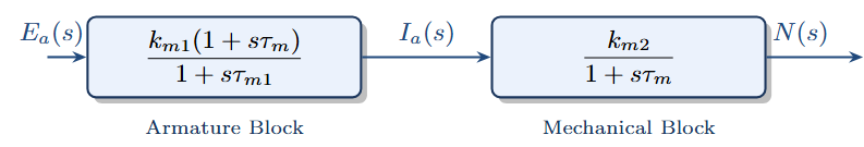
Simplified Motor Transfer Function
Neglecting \(T_L\) and using the full block-diagram representation:
Since \(\tau_a \ll \tau_m\), the electrical time constant may be neglected:
Two-Block Motor Representation
4. Closed-Loop Speed Control
- A DC tachogenerator attached to the motor shaft feeds back a speed signal.
- Speed error \(\varepsilon_N(s)\) controls the armature voltage.
- The armature voltage is regulated by a three-phase full converter.
Converter gain (cosine firing — linear relationship):
where \(\hat{E}_c\) corresponds to 0° firing angle and \(V_{LL}\) is the AC line-to-line RMS voltage.
General closed-loop transfer function:
Proportional (P) Controller
Resulting closed-loop transfer function:
If \(k_s k_c k_{m1} k_{m2} k_t \gg 1\) (high loop gain):
P Controller — Current Response to Step Input
For a step change in \(E_r\), the time-domain current response is:
Normalising with respect to steady-state (\(\tau_m \gg \tau_1\)):
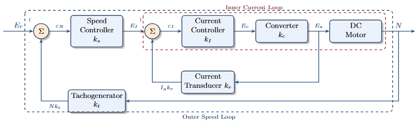
5. Current Control (Inner Loop)
Limitation of Pure Speed-Error Control
- Motor voltage is controlled by speed error alone.
- Clamping the speed error limits motor voltage, not current.
- If armature resistance is neglected, clamping limits speed, not current.
Solution
- Construct an inner current-control loop.
- Use the clamped speed-error signal as the current reference \(E_I\).
- Both P and PI controllers applicable to the current loop.
- \(k_r\) = gain of current transducer (sampling resistor)
- \(k_I\) = gain of current controller (proportional)
Current sensed → compared with \(E_I\) → error drives converter
Current Control — P Controller Transfer Function
For high inner-loop gain (\(k_r k_I k_c k_{m1} \gg 1\)) and since \(\tau_m \gg \tau_{m1}\):
Pole-Zero Cancellation
- Numerator zero at \(s = -1/\tau_m\)
- Denominator pole at \(s = -1/\tau_{m2} \approx -1/\tau_m\)
- Pole-zero cancellation is achieved → no overshoot, no time delay
- Armature electrical time constant \(\tau_a\)
- Converter delay
Speed Control with Inner Current Loop — P Controller
For \(k_t k_s k_{IC} k_{m2} \gg 1\):
Tachogenerator Filter — Effect on Transfer Function
A filter (time constant \(\tau_t\)) is sometimes needed to reduce ripple in the tachogenerator output. The resulting transfer function becomes second-order:
where \(k^{\prime} = (1 + k_s k_{IC} k_{m2} k_t) \simeq k_s k_{IC} k_{m2} k_t\).
6. Proportional-Integral (PI) Controller
- A P controller leaves a steady-state speed error.
- Adding integral action eliminates steady-state error and reduces the required forward gain.
PI controller transfer function: \(G_c(s) = \dfrac{k_s(1+\tau_s s)}{\tau_s s}\)
For \(k_t k_s k_{IC} k_{m2} \gg 1\), the overall closed-loop transfer function is:
where \(\tau_2 = \dfrac{\tau_m}{k_t k_s k_{IC} k_{m2}}\).
PI Controller — Current Response & P vs PI Comparison
Comparison: P vs PI Controller
| Feature | P | PI |
|---|---|---|
| Steady-state error | Yes | Zero |
| System order | 1st | 2nd |
| Overshoot | Low | Some |
| Speed recovery | Partial | Full |
Summary — Part 1
Key Concepts
- Closed-loop is essential for constant-speed drives.
- Motor has two time constants: \(\tau_a\) (electrical) and \(\tau_m\) (mechanical); typically \(\tau_a \ll \tau_m\).
- Motor represented by two transfer-function blocks.
- P controller: first-order, but large transient current.
- Inner current loop essential to limit overcurrent.
- With current loop, pole-zero cancellation gives clean response.
- PI controller: second-order, zero steady-state speed error.
Motor (simplified):
P controller (speed loop):
With current loop + PI:
System Design, Load Disturbances & Series Motor
1. Load Torque Disturbance Analysis
Practical Scenario
- In many applications a load is suddenly applied to the motor.
- The closed-loop system must reject this disturbance and restore speed.
- Both P and PI controllers are analysed.
Analysis Approach
- Changes in speed reference \(E_r\) are neglected.
- An expression for current is written in terms of speed change \(N(s)\).
- Full block diagram (with tachogenerator filter) is used.
P Controller — Speed Response to Load Disturbance
where \(\;k^\prime = 1 + \dfrac{K_a\Phi k_s k_t}{k_r B} = 1 + k_s k_t k_{IC} k_{m2}\). Since \(\dfrac{K_a\Phi k_s k_t}{k_r B} \gg 1\):
P Controller — Current Response to Load Disturbance
- Second-order response in both speed and current.
- Speed dips transiently and recovers.
- Current rises to supply the additional load torque.
- A steady-state speed error remains (characteristic of P control).
PI Controller — Speed Response to Load Disturbance
Replace the proportional gain \(k_s\) with the PI transfer function \(k_s\!\left[\dfrac{1+\tau_s s}{\tau_s s}\right]\). Because the PI controller provides filtering, the tachogenerator filter \(\tau_t\) may be omitted:
where \(\;\tau_2 = \dfrac{\tau_m k_r B}{K_a\Phi k_s k_t} = \dfrac{\tau_m}{k_{IC}k_{m2}k_s k_t}\).
Current Limiting During Start-Up
- Implemented via the inner current-control loop.
- Speed error is clamped at maximum value \(\hat{E}_I\).
- Current is therefore limited to \(\hat{I}_a = k_{IC}\hat{E}_I\).
- Once desired speed is reached, normal operation resumes.
If viscous friction \(B\) is very small:
2. Design Procedure for Closed-Loop Speed Control
System: 110 V, 2.5 hp, 1800 rpm separately excited DC motor.
| Parameter | Value | Parameter | Value |
|---|---|---|---|
| \(R_a\) | 1 Ω | \(J\) | 0.093 kg-m² |
| \(L_a\) | 46 mH | \(B\) | 0.008 N-m-s/rad |
| \(I_a\) (rated) | 20 A | \(K_a\Phi\) | 0.55 V-s/rad |
| \(\tau_a = L_a/R_a\) | 46 ms | \(\tau_m = J/B\) | 11.63 s |
| \(\tau_t\) | 0.1 s | \(\tau_{m1}\) | 0.3 s |
| \(k_{m1}\) | 0.0258 A/V | \(k_{m2}\) | 68.75 rad/s-A |
| \(k_t\) | 0.057 V-s/rad | \(k_r\) | 0.5 V/A |
| \(k_c\) | 25 | \(k_{IC} \simeq 1/k_r\) | 2 |
Design Step 1 — Current Controller Gain \(k_I\)
Based on steady-state error \(\varepsilon_I(\infty)\) of the current-control loop:
Numerical calculation for \(\varepsilon_I(\infty) = 10\%\):
Design Step 2 — Current Limit Reference \(\hat{E}_I\)
Numerical calculation for a current limit of 25 A:
Design Step 3a — Speed Controller Gain \(k_s\) (P Controller)
Numerical calculation for 0.25% steady-state speed error (\(\varepsilon_N(\infty) = 0.0025\)):
Design Step 3b — Speed Controller Gain \(k_s\) (PI Controller)
For the PI controller, steady-state speed error is ideally zero. Design is based on damping ratio and natural frequency.
Characteristic equation: \(1 + s\tau_s + s^2\tau_s\tau_2 = 0\)
Poles: \(s = \dfrac{1}{2\tau_2}\left[-1 \pm j\sqrt{\dfrac{4\tau_2}{\tau_s}-1}\right]\)
Commonly accepted damping ratio \(= 1/\sqrt{2}\), which requires: \(\tau_s = 2\tau_2\)
PI Design — Numerical Calculation
Choose \(\omega_n = 10\;\text{rad/s}\). Then:
| Controller | \(k_s\) | Speed Error | Response |
|---|---|---|---|
| P | 51 | 0.25% (residual) | 1st order (with filter: 2nd order) |
| PI | 21 | 0% (ideal) | 2nd order |
3. Series DC Motor Model
Applications
- Best suited for vehicle, crane, and hoist drives.
- Large starting torques at low speeds are required.
- If the circuit saturates, flux per pole is essentially constant ⟹ behaviour similar to separately excited motor.
- Product term: \(K_{af}i_a n\)
- Square term: \(K_{af}i_a^2\)
- Parameter variation: \(R_a, L_a, K_{af}, B\)
- Linearized model — valid for small-signal perturbations around a steady-state operating point.
- Numerical method — rigorous, valid for large disturbances.
Linearized Model
Average-value governing equations (inductance voltage averages to zero):
Small-signal perturbation around operating point \((I_{ao},\,N_o)\):
Laplace Domain & Block Diagram
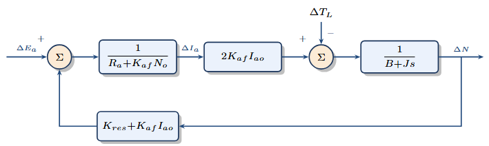
Step Change in Motor Voltage (\(\Delta T_L = 0\))
Step Change in Load Torque (\(\Delta E_a = 0\))
4. Numerical Analysis vs. Linearized Model
Why Numerical Analysis?
- Linearized model valid only for small disturbances around the operating point.
- Numerical method solves the nonlinear ODEs directly.
- Gives instantaneous variations of speed and current.
- Valid for small and large disturbances.
- Read motor and supply parameters.
- Initialise \(\omega t = 0\).
- Compute \(i_a\), \(n\) using R-K method.
- Check if one cycle is complete.
- Compute average/rms currents, speed, and torques.
- Check convergence (accel. torque < 0.001 pu).
- Output results; apply next disturbance.
Comparison Parameters
| Parameter | Value | Parameter / Value |
|---|---|---|
| \(K_{af}\) | 0.027 H | \(K_{res} = 0.0273\) V-s/rad |
| \(R_a\) | 1 Ω | \(L_a = 32\) mH |
| \(J\) | 0.0465 kg-m² | \(B = 0.004\) N-m-s/rad |
| Supply | 1ϕ, 120 V, 60 Hz | Converter: Semi-converter |
| Voltage change | \(\Delta E_a = 5.4\) V ≈ 5% | (\(\alpha\): 25.8° to 0°) |
| Torque change | \(\Delta T = 1\) N-m ≈ 10% | (\(T_L\): 9 to 10 N-m) |
Summary — Part 2
Key Concepts
- Load torque disturbances produce second-order responses under P control; poles are identical for speed-step and torque-step inputs.
- PI controller gives zero steady-state speed change for a step torque disturbance.
- Current limiting during start-up protects the converter; speed rises linearly under constant current.
- Design procedure: gains \(k_I\), \(k_s\) and limit \(\hat{E}_I\) chosen from steady-state error and damping requirements.
- Series motor equations are inherently nonlinear.
- Linearized model gives fair accuracy when validated against the Runge-Kutta numerical method.
Step voltage:
Step torque:
where \(\tau_o = J/B_o\), \(B_o > B\)
Modern Control — PLL & Microcomputer
1. Limitations of Analog Feedback Control
Shortcomings of Analog Control
- Speed sensing devices are not ideal.
- Other analog components in the feedback circuit are less than ideal.
- At best 0.2% speed regulation achievable.
- Transient speed dip when torque changes, with a delay before steady-state speed is restored.
- Not satisfactory in drives where high-quality products are required.
1. Phase-Locked-Loop (PLL) Control
- Digital technique; locks motor speed to a reference frequency.
- Speed regulation as low as 0.002% — hundredfold improvement over analog.
2. Microcomputer Control
- Eliminates analog component errors.
- Software-configurable control law.
- High accuracy, fast response, built-in fault diagnostics.
2. Phase-Locked-Loop (PLL) Control
Basic PLL Circuit
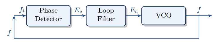
- Phase detector: digital IC; compares pulse trains \(f_i\) and \(f\); produces pulse-width modulated output \(E_e\) proportional to the phase difference.
- Loop filter: converts \(E_e\) to a DC level \(E_c\) representing the phase error.
- VCO: output frequency \(f\) changes in response to input voltage \(E_c\).
- If \(f_i = f\) and coincident: output is zero.
- If \(f\) lags \(f_i\): positive error \(E_e\).
- If \(f\) leads \(f_i\): negative error \(E_e\).
- If \(f > f_i\): continuous positive \(E_e\).
- If \(f < f_i\): continuous negative \(E_e\).
PLL Applied to Motor Speed Control
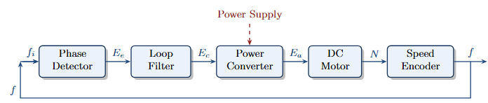
- The speed encoder generates a speed-dependent pulse train \(f\).
- \(f\) is compared with reference pulse train \(f_i\) (representing desired speed).
- Any speed deviation is detected almost instantaneously by the phase detector.
- As long as \(f = f_i\), steady-state speed is unaffected ⟹ theoretically perfect speed regulation.
PLL Transfer Function Model
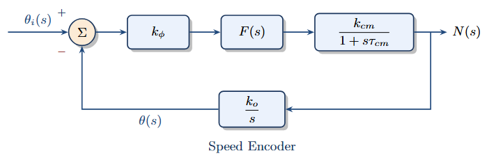
where \(G(s) = \dfrac{k_\phi k_{cm} F(s)}{1+s\tau_{cm}}\), \(H(s) = \dfrac{k_o}{s}\)
where \(k = k_\phi\, k_{cm}\, k_o\)
Converter-Motor Gain and Time Constant
Both gain and time constant are large.
Both gain and time constant are small.
Filter Transfer Function \(F(s)\) — Options & Stability
| Case | \(F(s)\) | Small motor (\(\tau_{cm}\) small) | Large motor (\(\tau_{cm}\) large) |
|---|---|---|---|
| 1 | \(\dfrac{1}{1+s\tau_1}\) (low-pass) | Stable at low gain; unstable at high gain | Unstable at smaller gain |
| 2 | \(\dfrac{1}{s}\) (integrator) | Unstable/oscillatory for all gains | Unstable/oscillatory for all gains |
| 3 | \(\dfrac{1+s\tau_1}{s}\) (PI) | Stable (leftward pole swing) | Not improved |
| 4 | \(\dfrac{1+s\tau_1}{1+s\tau_2},\;\tau_1>\tau_2\) (phase-lead) | Good; leftward swing | Leftward swing of dominant poles |
| 5 | \(s\) (derivative) | System does not remain phase-locked | System does not remain phase-locked |
| 6 | \(1+s\tau_1\) (PD) | Poles drawn left effectively | Stable with high gain |
Problem: Derivative feedback has high noise susceptibility.
Hybrid PLL Drive for Stable Operation
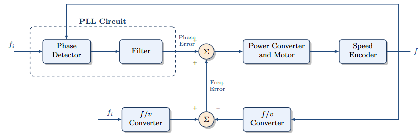
- Filter output ∝ phase error.
- Difference of \(f/v\) outputs ∝ frequency error (derivative of phase error).
- All three filters have approximately the same time constant.
PLL Drive — Practical Considerations
Pulses per Revolution
- For fast response, more pulses per revolution are required.
- More pulses allow use of a smaller filter time constant.
- A very large number of pulses results in high loop gain, which may create a stability problem.
- 36 to 120 pulses per revolution have been used in practical applications.
Applications
- Multi-motor synchronisation: conveyor systems.
- Digital clock coordination: computer peripherals.
- High-quality product drives: paper mills, textile mills, printing mills.
3. Microcomputer Control
Disadvantages of Analog Control
- Nonlinearity in analog speed transducer.
- Difficulty in accurately transmitting analog signals.
- Errors due to temperature and component aging.
- Drift and offset of analog components.
- Extraneous disturbances.
- Cannot handle complex, adaptive control functions.
Speed reference: set digitally.
Speed sensing: digital tachometer produces pulse train; frequency ∝ motor speed; fed to a digital counter.
Speed comparison: two digital counts compared in a gated comparator.
Speed error: drives an up/down counter; proportionality constant = gain of digital controller.
Basics of Microprocessors and Microcomputers
A microcomputer is a bus-oriented control unit interconnecting several LSI chips.
- Microprocessor (CPU): performs calculations and controls functions; executes instructions stored in memory.
- ALU: performs logical and arithmetic operations (addition, subtraction, bit manipulation).
- Data registers: intermediate data storage; reduce memory transfers.
- Address registers: store memory addresses; used for data transfer to/from memory.
- Control unit: supervises instruction execution; contains the clock.
| Data bus | 8 lines (8-bit µP) |
| Address bus | 16 lines |
| Control bus | 6 lines |
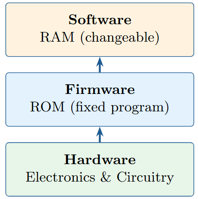
ROM — Instructions stored permanently (non-volatile); stores look-up tables and fixed programs.
RAM — Information can be written and read; stores data variables and changeable program portions.
I/O Interface, Buses and Software
Input-Output (I/O) Interface
- Permits communication between CPU and the outside world.
- Transfers data between CPU and external devices.
- Converts external data into a form usable by the microcomputer.
Software
- Microprocessor understands only binary codes.
- Programmer writes in assembly language.
- Assembler program converts symbolic source-program into binary object-program.
- Firmware: program held in ROM; not changeable by user.
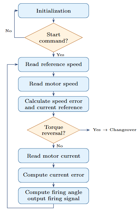
Microcomputer Control of Reversing Drives
- Speed input via DC tachometer + A/D converter or digital tachometer + digital counter.
- Motor current fed via fast A/D converter.
- Synchronising circuit: microprocessor synchronises firing pulses with supply line frequency.
- Gate pulse generator: receives firing signal from microcomputer; external logic generates firing pulses in proper sequence.
- Changeover logic: manages forward/reverse thyristor converter switching.
Stability and Performance
- Stability depends partly on the operating speed of the microprocessor.
- Mainly depends on how the standard analog controller scheme (P or PI) is implemented in software.
- Once I/O hardware is designed, a desired response is obtained by simply changing constants in the software control equations.
Example Applications
- Battery-powered electric vehicle: optimum torque control, regenerative and friction braking, battery charging, fault monitoring.
- Rolling mills, paper mills: high accuracy, good speed resolution, fast response.
- Blending of regenerative and friction braking.
- Programmed battery charging.
- Fault monitoring and diagnostics.
- Nonlinear functions stored as look-up tables.
- Supervisory monitoring from a central computer via high-speed digital transmission.
4. State of the Art — Microprocessor-Based Drives
Historical Milestone
- 1972: Intel first announced microprocessors.
- Most widely used: 8-bit microprocessors.
- Clock frequency range: 0.1 to 10 MHz.
Examples of 8-bit microprocessors:
Intel 8080 · Motorola 6800 · Fairchild F-8 · TI 9980 · RCA 1802 · Rockwell RPS-8 · Signetics 2650 · Zilog Z80
Advantages of Microprocessor-Based Drives
- Flexibility: change control scheme by modifying software only.
- Fully digital: decreased sensitivity to external disturbances.
- Fewer components: improved reliability and less wiring.
- Built-in fault-finding programs: diagnostic programs isolate faulty boards.
- Nonlinear functions: stored as look-up tables in memory.
- High accuracy, better time response, better speed regulation.
- Remote monitoring via digital high-speed transmission.
Future Outlook
- Drives that require high levels of performance.
- Drives that receive commands from central computers.
- Or both.
| Hardwired Logic | Microcomputer |
|---|---|
| Simple control only | Complex control |
| Not flexible | Highly flexible |
| Difficult to upgrade | Software update only |
| No self-diagnosis | Built-in diagnostics |
| Analog errors | Fully digital |
Summary — All Three Parts
PLL Control — Key Points
- Motor speed converted to a digital pulse train; locked to a reference frequency.
- Phase detector + loop filter + power converter + motor + speed encoder form the closed loop.
- Filter \(F(s)\) choice is critical: PI filter for small motor; PD or phase-lead for large motor.
- Hybrid PLL + analog scheme gives theoretically zero speed regulation.
- Speed regulation as low as 0.002%; hundredfold improvement over analog.
- Suitable for multi-motor synchronised drives.
Microcomputer Control — Key Points
- Eliminates all analog component errors.
- Same outer speed + inner current loop structure, implemented in software.
- Digital tachometer, A/D converter, digital counter for speed and current sensing.
- Stability governed by how P/PI is implemented in software.
- Handles complex tasks: nonlinear functions via look-up tables, fault diagnostics, remote monitoring.
- As cost falls, will become standard in high-performance industrial drives.