Coupled electromechanical equations:
Dynamic Model
Today's focus:
- Transform time-domain equations to frequency domain
- Derive transfer functions for system analysis
- Develop complete block diagram representation
- State-space modeling approach
- Stability analysis and system characteristics
Laplace Transform Approach
Advantages of frequency domain analysis:
Time Domain:
- Differential equations
- Complex to solve
- Hard to visualize system behavior
- Numerical methods often needed
Frequency Domain:
- Algebraic equations
- Easier manipulation
- Clear system properties
- Transfer functions reveal characteristics
Laplace Transform
where \(s = \sigma + j\omega\) is the complex frequency variable
Key property: \(\mathcal{L}\left\{\dfrac{df}{dt}\right\} = sF(s) - f(0^-)\)
Armature equation:
Taking Laplace transform (assuming zero initial conditions):
Mechanical equation:
Taking Laplace transform:
From armature equation:
Solving for \(I_a(s)\):
Current Expression
This can be written as:
Electrical impedance: \(Z_a(s) = R_a + sL_a\)
From mechanical equation:
Solving for \(\Omega_m(s)\):
Speed Expression
Interpretation:
- First term: Speed response to electromagnetic torque
- Second term: Speed response to load disturbance
Mechanical impedance: \(Z_m(s) = Js + B\)
Block Diagram Development
From \(I_a(s) = \dfrac{V(s) - K_e\Omega_m(s)}{R_a + sL_a}\)
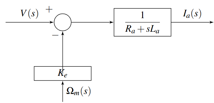
Interpretation:
- Input voltage \(V(s)\) drives the armature circuit
- Back-EMF \(K_e\Omega_m(s)\) opposes the applied voltage
- Net voltage across impedance determines current
From \(\Omega_m(s) = \dfrac{K_t I_a(s) - T_L(s)}{Js + B}\)
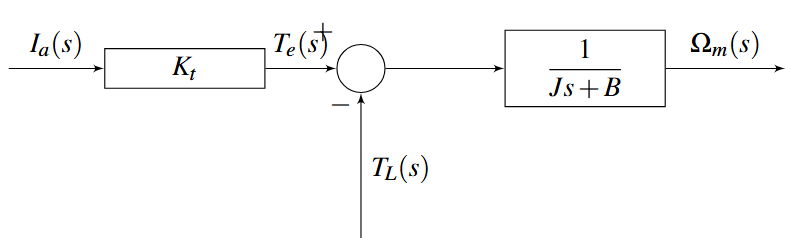
Interpretation:
- Armature current produces electromagnetic torque \(T_e = K_t I_a\)
- Net torque (electromagnetic minus load) accelerates the rotor
- Mechanical dynamics relate net torque to speed
Combining electrical and mechanical subsystems:
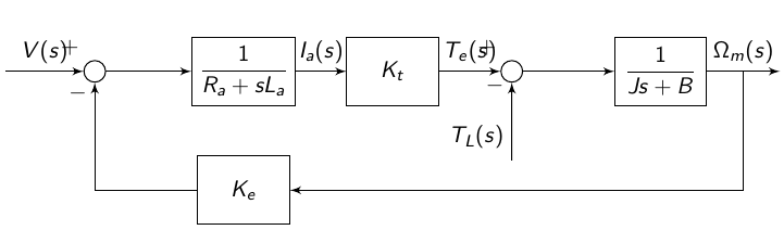
Key observation: The back-EMF provides negative feedback, which is crucial for stability and speed regulation.
Transfer Function Derivation
Goal: Find \(G_v(s) = \dfrac{\Omega_m(s)}{V(s)}\) with \(T_L(s) = 0\)
From the two equations:
From equation (2):
Substituting into equation (1):
Expanding the numerator:
Voltage-to-Speed Transfer Function
Goal: Find \(G_L(s) = \dfrac{\Omega_m(s)}{T_L(s)}\) with \(V(s) = 0\)
From the equations with \(V = 0\):
From first equation:
Substituting into second equation:
Load-to-Speed Transfer Function
Standard second-order form:
Comparing with our transfer function:
System Parameters
Natural frequency:
Damping ratio:
DC gain:
Natural frequency \(\omega_n\):
- Characterizes how fast the system responds
- Higher \(\omega_n\) means faster response
- Depends on electrical and mechanical parameters
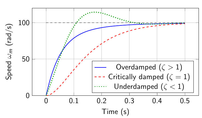
Damping ratio \(\zeta\):
- \(\zeta < 1\): Underdamped (oscillatory response)
- \(\zeta = 1\): Critically damped
- \(\zeta > 1\): Overdamped (slow, non-oscillatory)
- Most DC motors are overdamped
DC gain \(K_{dc}\):
- Steady-state speed per unit voltage
- Units: (rad/s)/V
- Important for speed control design
For many DC motors, we can identify two time constants:
Electrical Time Constant
Determines how fast the current responds to voltage changes
Mechanical Time Constant
Determines how fast the speed responds to torque changes
Typical relationship: \(\tau_m \gg \tau_e\)
The mechanical response is much slower than the electrical response
State-Space Modeling
Advantages over transfer functions:
- Can handle multiple inputs and outputs (MIMO systems)
- Works for time-varying and nonlinear systems
- Direct access to all internal states
- Foundation for modern control design
- Better for computer implementation
State-Space Form
where:
- \(\mathbf{x}\): State vector
- \(\mathbf{u}\): Input vector
- \(\mathbf{y}\): Output vector
- \(\mathbf{A, B, C, D}\): System matrices
Choose states that completely describe the system:
State Variables
- \(I_a\): Armature current (A)
- \(\omega_m\): Motor speed (rad/s)
Input Variables
- \(V\): Applied voltage (V)
- \(T_L\): Load torque (N·m)
Output: Typically \(y = \omega_m\) (speed measurement)
Starting from the dynamic equations:
Solving for derivatives:
In matrix form:
State Equation
Output Equation
If output is speed:
Identifying the matrices:
State Matrix A
Describes system dynamics
Input Matrix B
Describes how inputs affect states
Output Matrix C
Selects speed as output
Feedthrough Matrix D
No direct feedthrough from input to output
Stability Analysis
System stability determined by eigenvalues of \(\mathbf{A}\):
Expanding the determinant:
Stability Condition
System is stable if all eigenvalues have negative real parts
For DC motor: Always stable since all parameters are positive
The characteristic equation is:
This is identical to the denominator of our transfer function!
Poles determine system response:
- Real, negative poles → Exponential decay
- Complex conjugate poles → Damped oscillation
- Location determines speed of response
Key performance metrics:
- Rise time \(t_r\): Time to reach 90% of final value
- Settling time \(t_s\): Time to stay within 2% of final value
- Peak time \(t_p\): Time to first peak (if oscillatory)
- Overshoot \(M_p\): Maximum overshoot percentage
Most DC motors exhibit overdamped response: smooth approach to steady-state without oscillation.
At steady-state, all derivatives are zero:
From the state equations with \(\dfrac{dI_a}{dt} = 0\) and \(\dfrac{d\omega_m}{dt} = 0\):
Solving for steady-state speed:
Steady-State Speed
Speed regulation quantifies how speed changes with load:
Speed Regulation Definition
where nl = no-load, fl = full-load
From steady-state equation:
Speed drop per unit load torque:
Design Insight
For better speed regulation (less speed drop with load):
- Increase \(K_e\) and \(K_t\) (stronger magnetic field)
- Decrease \(R_a\) (lower armature resistance)
Example Problem
Given a separately-excited DC motor with parameters:
- Armature resistance: \(R_a = 2~\Omega\)
- Armature inductance: \(L_a = 0.01\) H
- Back-EMF constant: \(K_e = K_t = 0.5\) V/(rad/s) = 0.5 N\(\cdot\)m/A
- Moment of inertia: \(J = 0.02\) kg\(\cdot\)m\(^2\)
- Viscous friction: \(B = 0.001\) N\(\cdot\)m\(\cdot\)s/rad
Tasks:
- Calculate the time constants \(\tau_e\) and \(\tau_m\)
- Determine the natural frequency \(\omega_n\) and damping ratio \(\zeta\)
- Find the steady-state speed for \(V = 100\) V and \(T_L = 5\) N\(\cdot\)m
- Calculate the DC gain \(K_{dc}\)
1. Time constants:
Note: \(\tau_m \gg \tau_e\) (mechanical response much slower)
2. Natural frequency and damping ratio:
System is heavily overdamped (no oscillations expected).
3. Steady-state speed:
4. DC gain:
This means the motor speed increases by approximately 2 rad/s for every 1 V increase in applied voltage at steady-state.
Transfer function models:
- Voltage-to-speed: \(G_v(s) = \dfrac{K_t}{JL_a s^2 + (BL_a + JR_a)s + (BR_a + K_e K_t)}\)
- Load-to-speed: \(G_L(s) = \dfrac{-(R_a + sL_a)}{JL_a s^2 + (BL_a + JR_a)s + (BR_a + K_e K_t)}\)
- Second-order system with parameters \(\omega_n\) and \(\zeta\)
State-space model:
- States: \([I_a, \omega_m]^T\) (current and speed)
- Inputs: \([V, T_L]^T\) (voltage and load torque)
- Complete description of system dynamics
- Suitable for modern control design
System characteristics:
- Inherently stable (all poles in left half-plane)
- Usually overdamped (\(\tau_m \gg \tau_e\))
- Natural speed regulation due to back-EMF feedback