Need for DC Motor Speed Control
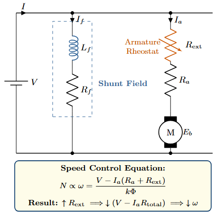
Fundamental Speed Equation
where \(V_a\) is armature voltage, \(I_a\) is armature current, \(R_a\) is armature resistance, \(K\) is machine constant, and \(\phi\) is field flux.
Speed Control Methods:
- Armature voltage control (\(V_a\))
- Field flux control (\(\phi\))
- Armature resistance control (\(R_a\))
DC Motor Drives are Essential in:
- Electric vehicles & traction systems
- Cranes and hoists
- Conveyor systems
- CNC machine tools
- Battery-powered equipment
- Renewable energy systems
- Solar pumping applications
- MPPT-based drives
Key Requirement
Modern applications demand efficient, precise, and responsive speed control with minimal energy losses.
Traditional Methods:
-
Rheostatic (resistance) control
- Variable resistance in series with armature
- Simple but inefficient
-
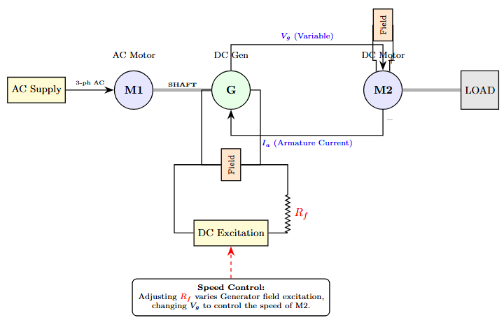
Motor-Generator (Ward-Leonard) set
- AC motor drives DC generator
- Variable voltage output
-
Phase-controlled rectifiers (SCR)
- AC to controlled DC conversion
- Thyristor-based control
Conventional Methods and Limitations
| Parameter | Rheostatic | M-G Set | SCR Rectifier | Chopper |
|---|---|---|---|---|
| Efficiency | Very poor (\(<50\%\)\)) | Moderate (60–75%) | Good (80–90%) | Excellent (\(>95\%\)\)) |
| Response time | Fast | Slow | Moderate | Very fast (ms) |
| Size/Weight | Compact | Very bulky | Compact | Compact |
| Maintenance | Minimal | High | Low | Minimal |
| DC source usable | Yes | No | No | Yes |
| Power factor | N/A | Good | Poor | N/A |
| Harmonics | None | None | Significant | Low |
Rheostatic Control
Disadvantages:
- Very poor efficiency (\(<50\%\)\))
- Energy wasted as heat in resistors
- Speed regulation poor under load
- Limited speed range
Ward-Leonard Set
Disadvantages:
- Very bulky and heavy
- High initial cost
- Slow dynamic response
- High maintenance (rotating machines)
Phase-Controlled Rectifier
Disadvantages:
- Poor power factor (especially at low speeds)
- Significant harmonic content
- Requires AC source (not suitable for battery/solar)
- Complex filtering needed
Modern Solution
DC choppers overcome all these limitations with high efficiency, fast response, and DC source compatibility.
Motivation for DC Chopper Drives
Modern drive applications demand: high efficiency, fast dynamic response, DC-source compatibility, compact form factor, and low maintenance.
Choppers deliver all five requirements.
Key Advantages
- Efficiency \(> 95\%\)
- Fast dynamic response (millisecond range)
- Compact and lightweight design
- Compatible with DC sources (batteries, solar panels)
- Low maintenance (no moving parts)
Application Domains
- Electric and hybrid vehicles
- Battery-powered equipment
- Solar PV pumping systems
- Traction systems
- Industrial servo drives
DC Chopper: Operating Principle
Definition
A DC chopper is a static power electronic device that converts a fixed-voltage DC source into a variable-voltage DC output through high-frequency switching of a power semiconductor device (MOSFET, IGBT, GTO, etc.).
DC Transformer Analogy
A DC chopper is analogous to an AC transformer with a continuously variable turns ratio, but it operates on DC voltage and achieves step-up or step-down conversion with high efficiency (\(>95\%\)\)).
Key Principle:
- Energy transfer through switching (not resistive dissipation)
- Output voltage controlled by duty cycle
- No moving parts \(\Rightarrow\) high reliability
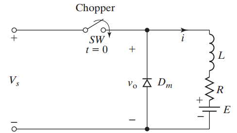
Components:
- \(Q\): Power switch (MOSFET/IGBT)
- \(D_m\): Freewheeling diode
- \(L_a\): Armature inductance
- \(V_s\): DC source voltage
Operation
When \(Q\) is ON: motor connected to source
When \(Q\) is OFF: current freewheels through \(D_m\)
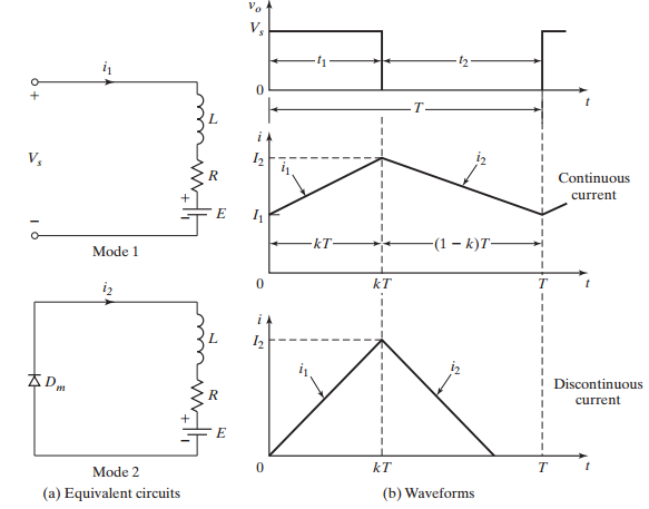
Two Switching States:
State 1: Switch ON (\(t_{\text{ON}}\))
- Current path: \(V_s \to Q \to\) Motor
- Motor voltage: \(v_a = V_s\)
- Energy supplied from source
- Armature current increases
State 2: Switch OFF (\(t_{\text{OFF}}\))
- Current path: Motor \(\to D_m\)
- Motor voltage: \(v_a \approx 0\)
- Energy stored in inductance
- Armature current decreases
Average Output Voltage
where \(k\) is the duty cycle: \(k = \dfrac{t_{\text{ON}}}{T}\), \(0 \le k \le 1\)
Duty Cycle Definition
where \(T\) is the chopping period and \(f = 1/T\) is the chopping frequency.
Voltage Relationships:
- \(k = 0\): \(V_a = 0\) (motor stopped)
- \(k = 0.5\): \(V_a = 0.5 V_s\)
- \(k = 1\): \(V_a = V_s\) (full speed)
Speed control achieved by varying \(k\) from 0 to 1.
Typical Parameters:
- Chopping frequency: 1–20 kHz
- Duty cycle range: 0–100%
- Linear voltage control
- Continuous current mode preferred
Step-Down (Buck) Chopper: Circuit and Waveforms
Characteristics:
- Also called Buck chopper
- Output voltage: \(V_a = k V_s\)
- \(0 \le k \le 1\)
- Power flow: source \(\to\) load
Applications:
- DC motor speed control
- Battery charging
- Voltage regulators
Current Ripple
Design Consideration
Higher chopping frequency \(\Rightarrow\) Lower current ripple \(\Rightarrow\) Smoother motor operation
Continuous Conduction Mode (CCM)
- Current never falls to zero
- \(I_{\min} > 0\)
- Better for motor control
- Requires: \(L_a > L_{\text{critical}}\)
Discontinuous Conduction Mode (DCM)
- Current falls to zero during OFF period
- \(I_{\min} = 0\)
- Higher current ripple
- Occurs at light loads or low \(L_a\)
Effect:
- Non-linear control
- Higher torque ripple
- Generally avoided in motor drives
Average Armature Voltage
Average Armature Current (Steady State)
where \(E\) is the back-EMF of the motor.
Power Relationships:
- Input power: \(P_{\text{in}} = V_s I_s\)
- Output power: \(P_{\text{out}} = V_a I_a = k V_s I_a\)
- Efficiency: \(\eta = \dfrac{P_{\text{out}}}{P_{\text{in}}} > 95\%\) (typical)
Step-Up (Boost) Chopper: Circuit
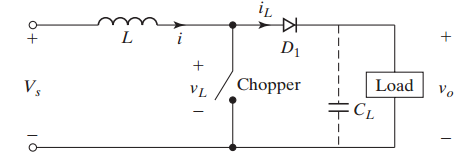
Characteristics:
- Also called Boost chopper
- Output voltage: \(V_a = \dfrac{V_s}{1-k}\)
- \(V_a > V_s\) (voltage boost)
- \(0 \le k < 1\)
Operating Principle:
- When \(Q\) ON: Energy stored in \(L\)
- When \(Q\) OFF: \(L\) releases energy
- Voltage across \(L\) adds to \(V_s\)
- Diode prevents reverse flow
Application
Used for regenerative braking in DC motor drives
Voltage Boost Relationship
where \(k\) is the duty cycle.
Examples:
- \(k = 0.5\): \(V_a = 2 V_s\) (voltage doubled)
- \(k = 0.75\): \(V_a = 4 V_s\) (four times boost)
- \(k \to 1\): \(V_a \to \infty\) (theoretical limit)
Practical Limitation
In practice, \(k\) is limited to 0.8–0.9 due to switching losses and component limitations. Typical boost ratio: 2–5 times.
Braking Operation:
- Motor acts as generator
- Back-EMF \(E > V_s\)
- Energy returned to source
- Current flows from motor to source
Power Flow
Energy recovered in battery/capacitor
Applications:
- Electric vehicles (downhill braking)
- Cranes (lowering loads)
- Elevators (descending)
- Traction systems
Efficiency Benefit
Regenerative braking can recover 60–70% of kinetic energy, significantly improving overall system efficiency.
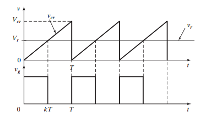
Pulse Width Modulation (PWM)
PWM Principle
Advantages:
- Constant switching frequency
- Linear voltage control
- Low harmonic content
- Easy digital implementation
- Predictable filtering requirements
Parameters:
- Carrier frequency: \(f_c\) (1–20 kHz)
- Modulation index: \(m = V_{\text{control}}/V_{\text{carrier}}\)
- Duty cycle: \(k = m\)
- Output voltage: \(V_a = m V_s\)
Analog PWM
- Compare control signal with triangular carrier
- Op-amp based comparator
- Continuous modulation
- Simple hardware
Digital PWM
- Microcontroller/DSP based
- Timer/counter implementation
- Programmable frequency and duty cycle
- Flexible and precise
Update \(k\) based on feedback control
Modern Practice
Digital PWM is the industry standard due to flexibility, programmability, and integration with control algorithms.
Constant Frequency (PWM)
Features:
- Fixed period \(T\)
- Variable \(t_{\text{ON}}\)
- Duty cycle: \(k = t_{\text{ON}}/T\)
Advantages:
- Predictable harmonics
- Easy filtering
- Linear control
- Preferred method
Variable Frequency
Features:
- Fixed \(t_{\text{ON}}\) or \(t_{\text{OFF}}\)
- Variable period \(T\)
- Frequency modulation
Disadvantages:
- Variable harmonics
- Complex filtering
- Non-linear control
- Rarely used in motor drives
Trade-offs in Choosing Switching Frequency:
Higher Frequency (>10 kHz)
Advantages:
- Lower current ripple
- Smoother torque
- Smaller filter components
- Quieter operation (above audible range)
Disadvantages:
- Higher switching losses
- Increased EMI
- More expensive switches
Lower Frequency (1–5 kHz)
Advantages:
- Lower switching losses
- Higher efficiency
- Less EMI
- Lower cost switches
Disadvantages:
- Higher current ripple
- Larger inductors needed
- Audible noise
- Greater torque ripple
Typical Range: 2–20 kHz depending on power level and application
Current Ripple Analysis
Peak-to-Peak Current Ripple
where \(f = 1/T\) is the switching frequency.
Maximum Ripple Condition:
- Maximum ripple occurs at \(k = 0.5\) (50% duty cycle)
- At this point: \(\Delta I_{\max} = \dfrac{V_s}{4 f L_a}\)
Design Implication
Inductance \(L_a\) must be sized for worst-case ripple at \(k = 0.5\) to ensure CCM throughout the operating range.
Critical Inductance
where the maximum value occurs at \(k = 0.5\).
where \(\Delta I_{\max}\) is the maximum allowable current ripple.
Typical Design Rule:
- Limit ripple to 10–20% of rated current
- Example: For \(I_{\text{rated}} = 10\) A, choose \(\Delta I_{\max} = 1\)–2 A
- Calculate \(L_a\) accordingly
Given Data:
- Source voltage: \(V_s = 200\) V
- Switching frequency: \(f = 10\) kHz
- Rated current: \(I_{\text{rated}} = 20\) A
- Desired ripple: \(\Delta I_{\max} = 2\) A (10% of rated)
Design Choice:
- Select standard value: \(L_a = 3\) mH
- Add 20% safety margin
- Verify thermal and saturation ratings
Need for Input Filtering
Why Input Filters are Required:
Problems Without Filtering
- Pulsating input current
- High-frequency ripple
- EMI to source and other equipment
- Voltage spikes
- Source voltage variations
Filter Benefits
- Smooth DC input current
- Reduced EMI
- Protection of source
- Improved power quality
- Compliance with EMC standards
Standard Practice
An LC input filter is essential for all chopper drives, especially when powered from batteries or sensitive DC sources.
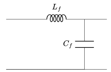
Filter Components:
- \(L_f\): Series inductor
- \(C_f\): Shunt capacitor
- Forms low-pass filter
Design Criteria
Additional Consideration:
- Damping resistor may be needed
- Prevents resonance oscillations
Design Equations
Practical Design Steps:
- Choose \(f_c = f_s/10\) to \(f_s/20\)
- Select capacitor \(C_f\) based on voltage ripple requirement:
\[C_f \ge \frac{I_{\text{rated}}}{2 \pi f_c \Delta V_{\text{ripple}}}\]
- Calculate inductor: \(L_f = \dfrac{1}{(2\pi f_c)^2 C_f}\)
- Verify inductor current rating \(\ge I_{\text{rated}}\)
- Add damping if needed to control resonance
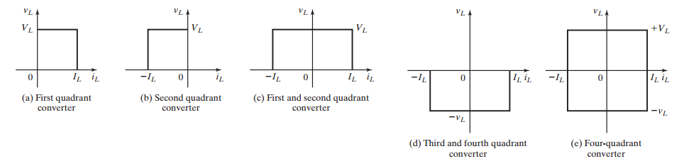
Classification of DC Choppers
Choppers are classified based on quadrant of operation:
| Class | Configuration | Quadrants | Application |
|---|---|---|---|
| A | Step-down (Buck) | Q1 (Forward motoring) | Basic speed control |
| B | Step-up (Boost) | Q2 (Forward braking) | Regenerative braking |
| C | Two-quadrant (A+B) | Q1, Q2 | Motoring + braking |
| D | Two-quadrant | Q1, Q4 | Bidirectional current |
| E | Four-quadrant (H-bridge) | Q1, Q2, Q3, Q4 | Full reversibility |
Selection Criteria
Choose chopper class based on application requirements: unidirectional vs. bidirectional operation, regenerative braking capability, and reversing requirements.
Operating Characteristics:
- Quadrant 1 only (Q1)
- \(v_a > 0\), \(i_a > 0\)
- Forward motoring only
- No braking capability
Voltage Control
where \(k\) is the duty cycle.
Applications:
- Simple DC motor drives
- Fan speed control
- Pump drives
- Unidirectional conveyors
Limitation: Cannot provide braking; motor coasts to stop when power is removed.
Operating Characteristics:
- Quadrant 2 only (Q2)
- \(v_a > 0\), \(i_a < 0\)
- Regenerative braking only
- Power flows: motor \(\to\) source
Voltage Boost
Back-EMF \(E > V_s\) required for regeneration.
Applications:
- Regenerative braking systems
- Energy recovery in EVs
- Hoist lowering operations
- Downhill traction
Note: Always used in combination with Class A for complete drive functionality.
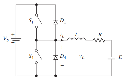
Structure:
- Combines Class A (\(Q_1\), \(D_1\)) and Class B (\(Q_2\), \(D_2\))
- Two power switches
- Bidirectional current capability
Operating Modes
Applications:
- Electric vehicles
- Traction systems
- Hoist drives
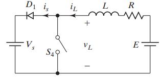
Operating Quadrants:
- Q1: Forward motoring (\(v_a > 0\), \(i_a > 0\))
- Q4: Reverse braking (\(v_a < 0\), \(i_a > 0\))
Voltage Reversal Capability
- Can reverse voltage polarity
- Current remains positive
- Enables field weakening
- Useful for special applications
Control Strategy:
- \(Q_1\) ON: \(v_a = +V_s\)
- \(Q_4\) ON: \(v_a = -V_s\)
- PWM modulation of \(Q_1\) and \(Q_4\)
Application: Specialized drives requiring voltage polarity reversal.
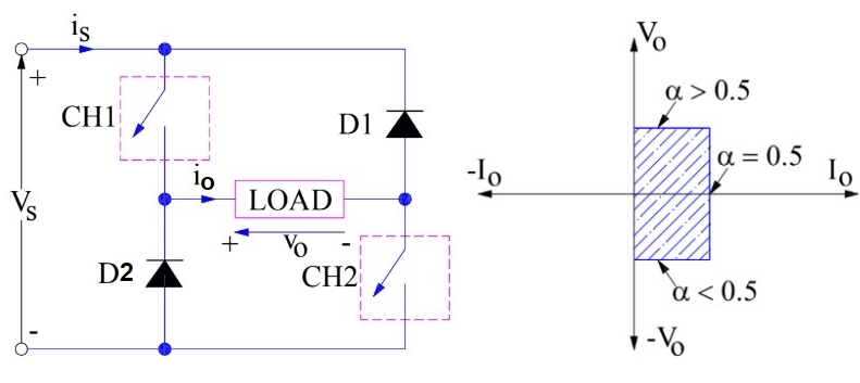
Mode 1: Forward Operation (\(\alpha > 0.5\))
- Switch \(Q_1\) ON for time \(t_a\)
- Switch \(Q_4\) ON for time \(T_p - t_a\)
- Average voltage:
For \(t_a > T_p/2\): \(\bar{v}_a > 0\) (motoring)
Duty cycle: \(\alpha = t_a/T_p\)
Mode 2: Reverse Operation (\(\alpha < 0.5\))
- Same switching pattern
- Different average voltage polarity
For \(t_a < T_p/2\): \(\bar{v}_a < 0\) (braking)
Transition Point
Current continues to flow, but average voltage is zero.
Converter Voltage Gain
Operating Regions:
- \(\alpha > 0.5\): \(\bar{v}_a > 0\)
- Power flow: source \(\to\) load
- Motoring operation
- \(\alpha = 0.5\): \(\bar{v}_a = 0\)
- Zero average voltage
- Current can be non-zero
- \(\alpha < 0.5\): \(\bar{v}_a < 0\)
- Power flow: load \(\to\) source
- Braking operation
Note
Current direction remains positive in both modes; only average voltage (and power flow) reverses.
Class E: Four-Quadrant H-Bridge Drive
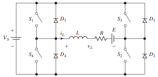
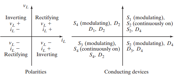
Structure:
- H-bridge configuration
- Four switches: \(Q_1\)–\(Q_4\)
- Four anti-parallel diodes: \(D_1\)–\(D_4\)
| Quadrant | \(v_L\) | \(i_L\) |
|---|---|---|
| Q1 (Fwd motoring) | \(+\) | \(+\) |
| Q2 (Fwd braking) | \(+\) | \(-\) |
| Q3 (Rev motoring) | \(-\) | \(-\) |
| Q4 (Rev braking) | \(-\) | \(+\) |
Configuration Flexibility:
- \(Q_4\) ON continuously \(\Rightarrow\) Class C behavior
- \(Q_1\), \(Q_2\) modulate for motoring/braking
- \(Q_1\) ON continuously \(\Rightarrow\) Class D behavior
- \(Q_3\), \(Q_4\) modulate for voltage reversal
Unified Topology
Class E subsumes Classes C and D by appropriate switching strategies. It is the most general and versatile topology.
Safety Constraints:
- \(Q_1\) and \(Q_2\) must never be ON simultaneously
- Causes shoot-through (short circuit)
- \(Q_3\) and \(Q_4\) must never be ON simultaneously
- Causes shoot-through
- Dead-time insertion: typically 1–5 \(\mu\)s
- Ensures safe commutation
- Prevents overlap
Complete Quadrant Coverage
Class E provides access to all four quadrants, enabling:
- Forward and reverse motoring
- Regenerative braking in both directions
- Seamless transitions between modes
Applications Requiring Four-Quadrant Operation:
- Reversible machine tools and CNC equipment
- Servo drives with bidirectional positioning
- Electric vehicle traction (forward/reverse with regeneration)
- Elevator drives (up/down with energy recovery)
- Rolling mill drives
- Test stands and dynamometers
Control Complexity
Four-quadrant operation requires sophisticated control algorithms to manage transitions and ensure stability across all operating modes.
Power Switching Devices for Choppers
| Device | Power Range | Freq. Range | Commutation | Typical Use |
|---|---|---|---|---|
| MOSFET | \(< 10\) kW | 20–100 kHz | Self-commutated | Low-power, high-freq |
| IGBT | 10–500 kW | 5–20 kHz | Self-commutated | Industrial standard |
| GTO | 100–5000 kW | 1–5 kHz | Self-commutated | High-power traction |
| Thyristor (SCR) | \(> 500\) kW | \(< 1\) kHz | Forced commutation | Legacy/very high power |
Selection Criteria:
- Power level of application
- Required switching frequency
- Voltage and current ratings
- Gate drive complexity
- Cost and availability
Self-Commutated Devices
Examples: MOSFET, IGBT, GTO
Characteristics:
- Turn ON and OFF controlled by gate signal
- No auxiliary circuit needed for turn-off
- Fast switching capability
- Simpler drive circuits
- Higher reliability
Status:
- Preferred for all modern drives
- Dominant in industrial applications
Forced-Commutated Devices
Example: Thyristor (SCR)
Characteristics:
- Gate controls only turn-ON
- External circuit required for turn-off
- Complex commutation circuits
- Adds cost and components
- Lower switching frequency
Status:
- Legacy technology
- Limited to very high power (\(>500\) kW)
- Being phased out
Why IGBT?
IGBT (Insulated Gate Bipolar Transistor) is the dominant device for industrial DC chopper drives in the 10–500 kW power range.
IGBT Advantages:
- High voltage capability (up to 6.5 kV)
- High current capability (up to 3600 A)
- Moderate switching frequency (5–20 kHz)
- Low on-state voltage drop
- Simple gate drive (voltage-controlled)
- Excellent safe operating area (SOA)
- Good thermal characteristics
Comparison with Alternatives:
- vs. MOSFET: Higher power capability
- vs. GTO: Simpler gate drive, higher frequency
- vs. SCR: Self-commutated, no turn-off circuit
Typical Ratings:
- Voltage: 600 V to 6.5 kV
- Current: 10 A to 3600 A
- Switching frequency: 1–20 kHz
Summary: Motivation and Core Relations
Why Choppers?
Classical Methods Limitations:
- Rheostatic: Poor efficiency (\(<50\%\)\))
- M-G set: Bulky, slow, expensive
- SCR rectifier: Poor PF, AC source required
Chopper Advantages:
- Efficiency \(> 95\%\)
- Fast response (ms range)
- Compact, lightweight
- DC-source compatible
Core Relations
Chopper Classes
- Class A: Step-down, Q1 motoring
- Class B: Step-up, Q2 braking
- Class C: Q1+Q2, motoring/braking (EV, traction)
- Class D: Two-quadrant (Q1+Q4), voltage reversal
- Class E: Four-quadrant H-bridge, fully reversible
Control & Devices
PWM Control:
- Constant frequency preferred
- Variable duty cycle: \(k = V_{\text{cr}}/V_r\)
- Linear voltage control
Key Design Points:
- Higher \(f_s\) \(\Rightarrow\) lower ripple, higher loss
- Input LC filter essential
- IGBT: standard for 10–500 kW drives