Closed-Loop Control of DC Drives with Chopper

Introduction to Closed-Loop Control

The Shift to Closed-Loop Control

Open-Loop Limitations

No load compensation
Sensitive to aging/temperature
Drift in speed/position
Voltage fluctuation issues
No safety mechanisms

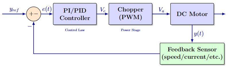
Closed-Loop Advantages

Self-correcting logic
High precision accuracy
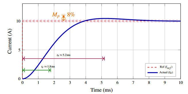
Faster settling times
Robust to variations
Built-in protection

Real-World Case: The Elevator

The motor must maintain speed regardless of the passenger load and stop perfectly level with the floor. Only closed-loop feedback ensures this reliability.

Closed-Loop Control of DC Drives

Core Principle

Closed-loop control automatically adjusts the duty cycle of the chopper to maintain a reference speed or torque by comparing actual output with desired setpoint and minimizing the error.

Essential Components:

Sensors: Measure actual speed (tachometer) and current (shunt/Hall-effect).
Comparator: Computes the error signal:
$$e(t) = y_{\text{ref}}(t) - y_{\text{measured}}(t)$$
Controller: Processes $e(t)$ via PI or PID algorithms.
Power Converter: The Chopper, which acts as the final actuator.

General feedback control structure block diagram showing reference input, comparator, controller, plant, and output feedback loop — General feedback control structure.

Control Variables ($y$)

Typically represents Speed ($\omega_m$), Armature Current ($i_a$), or Torque ($T_e$).

Purpose of Feedback Loops

Feedback loops satisfy three core operational objectives:

1. System Protection

Current Limiting: Prevents thermal damage.
Switch Safety: Avoids converter overcurrent.
Mechanical Safety: Prevents overspeed.
Regeneration: Overvoltage protection.

2. Dynamic Response

Settling Time: Faster steady-state.
Overshoot: Reduced oscillations.
Disturbance: Better rejection.
Tracking: Improved performance.

3. Static Accuracy

Error: Elimination of steady-state error.
Load Torque: Compensation for variations.
Parameters: Reduced sensitivity to changes.

Typical Control Variables in DC Drives

Torque/Current ($T_e = K_t i_a$) $\rightarrow$ Speed ($\omega_m$) $\rightarrow$ Position ($\theta$)
(Fastest / Innermost) (Slowest / Outermost)

Cascade Control Structure — Concept

Hierarchical Design

Cascade control arranges multiple nested feedback loops hierarchically, with faster inner loops and progressively slower outer loops, each controlling a specific variable.

Key Advantages:

Modularity: Tailor loops to application needs.
Natural Protection: Limit inner variables (e.g., current) easily.
Performance: Inner loops stabilize fast dynamics.
Design: Independent loop design via bandwidth separation.
Rejection: Rapid disturbance rejection.

Loop Dynamics & Bandwidths

Current/Torque Loop: $\tau_i \approx 1$–$5\,\text{ms}$, $f_{\text{BW}} \approx 100$–$1000\,\text{Hz}$
Speed Loop: $\tau_s \approx 10$–$100\,\text{ms}$, $f_{\text{BW}} \approx 10$–$100\,\text{Hz}$
Position Loop: $\tau_p \approx 100$–$1000\,\text{ms}$, $f_{\text{BW}} \approx 1$–$10\,\text{Hz}$

Design Rule: Bandwidth ratio between consecutive loops must be 5–10×.

Core Insight

Inner loops act as "pre-processors," stabilizing fast dynamics so outer loops see a simpler, slower system.

Cascade Control Structure — Implementation

Power Converter Options:

AC-DC Controlled Rectifier (Phase-controlled thyristor bridge)
DC-DC Converter (Chopper)
- Focus of this lecture

Nested loop hierarchy diagram showing position, speed, and current control loops arranged concentrically — Nested loop hierarchy.

Fundamental Design Principle

Design from inside out: Inner loops must be significantly faster than outer loops ($5$–$10\times$ bandwidth separation).

This ensures:

Settling: Inner dynamics settle before the outer loop acts.
Decoupling: Effective separation of different time-scale dynamics.
Stability: Guaranteed stability of the overall cascade.

DC Motor Fundamentals — Quick Review

Electrical Equation

$$V_a(t) = R_a i_a(t) + L_a \frac{di_a(t)}{dt} + e_b(t)$$

$e_b = K_b \omega_m$ (Back-EMF)

Parameters:

$V_a$: Armature voltage (V)
$R_a$: Armature resistance ($\Omega$)
$L_a$: Armature inductance (H)
$K_b$: Back-EMF constant (V·s/rad)

Mechanical Equation

$$T_e(t) = T_L(t) + J\frac{d\omega_m(t)}{dt} + B\omega_m(t)$$

$T_e = K_t i_a$ (Electromagnetic Torque)

Parameters:

$T_L$: Load torque (N·m)
$J$: Moment of inertia (kg·m²)
$B$: Friction coeff. (N·m·s/rad)
$K_t$: Torque constant (N·m/A)

Fundamental Relationships & Control Implication
$K_t = K_b$ (in consistent SI units)
$\omega_{ss} = \dfrac{V_a - R_a I_a}{K_b}$ (Steady-state speed)

              Key Takeaway:

              $\boxed{\text{Controlling } i_a \propto \text{Controlling } T_e}$
            

Motor Parameter Identification

Bridge from Theory to Hardware

Controller design depends on precise motor parameter identification, and the following are widely accepted industry methods for system modeling.

Electrical ($R$, $L$, $K$)

$R_a$ (DC Resistance)
Locked rotor; apply DC $V$; $R_a = V/I$.
Tip: Use low current to avoid heating.

$L_a$ (Inductance)
LCR meter at 1 kHz or AC impedance: $$L_a = \frac{\sqrt{Z^2 - R_a^2}}{\omega}$$

$K_e, K_t$ (Constants)
$K_e$: Open-circuit $V$ at known $\omega$.
$K_t$: Torque vs. Current slope.
Check: $K_t \approx K_e$ (in SI units).

Mechanical ($J$, $B$)

$J$ (Inertia)
Acceleration test: $J = T/\alpha$.
Or use CAD models/datasheets.

$B$ (Damping)
Coast-down test: Fit $\omega(t) = \omega_0 e^{-(B/J)t}$.
Often estimated from no-load current.

Validation Rules

$\tau_e = L_a/R_a$ ($\approx$ 1–10 ms)
$\tau_m = J/B$ ($\approx$ 50–500 ms)
$P_{out} \approx \frac{K_t K_e \omega^2}{R_a}$

Quick Estimate: $R_a$ (Multimeter) $\to$ $L_a$ (1–10 mH) $\to$ $K_t$ (Nameplate) $\to$ $B$ (Neglect)

Current Control Methods

Current Control for DC Drives with Choppers

Motivation for Current Control:

Torque Control: $T_e = K_t i_a$ directly links current to motion.
Dynamics: Enables precise control and fast response.
Protection: Inherent safety for motor and converter.
Hierarchy: Forms the innermost loop in cascade systems.

Industry Preference: PWM + PI

Overwhelmingly preferred due to predictable switching frequency, which simplifies EMI filter design and reduces electromagnetic interference.

In Chopper-based Drives:

Voltage Control: Chopper regulates $V_a = \delta V_{dc}$.
Dynamics: Armature voltage indirectly controls $i_a$.
Time Constant: Responds with $\tau_e = L_a/R_a$ (1–10 ms).

Strategies:

Hysteresis: Instantaneous bang-bang control.
PWM + PI: Fixed frequency, systematic design.

Hysteresis Current Control

Operating Principle

Compare actual $i_a$ with reference $i_a^*$.
ON State: $i_a < i_a^* - h \Rightarrow V_a = V_{dc}$.
OFF State: $i_a > i_a^* + h \Rightarrow V_a = 0$.
Hysteresis Band: $2h$ (current ripple).

Advantages:

Extremely fast dynamic response.
Simple implementation.
No controller tuning required.

Disadvantages:

Variable switching frequency.
Difficult EMI filter design.
Unpredictable acoustic noise.

Hysteresis current control waveform showing armature current oscillating within hysteresis band around reference current — Hysteresis Operation

Switching Frequency Analysis

For a step-down chopper ($V_{dc}$ to $0$):

$$f_s \approx \frac{V_{dc}(1-\delta)}{4hL_a}$$

where $\delta \approx e_b / V_{dc}$.

Note: Frequency varies with $V_{dc}$, $\omega_m$, and $L_a$, complicating optimization.

PWM-Based Current Control

Operating Principle

The PI controller minimizes the error: $e(t) = i_a^*(t) - i_a(t)$

Modulation: $v_c$ is compared to a triangular carrier $v_{\text{tri}}$.
Frequency: Fixed switching at $f_c$.

PWM Switching Logic

$v_c > v_{\text{tri}}$	$\Rightarrow$ Switch ON
$v_c < v_{\text{tri}}$	$\Rightarrow$ Switch OFF

Advantages:

Fixed $f_c$: Predictable EMI.
Linear control loop.
Industry standard.

PI-based PWM current control block diagram showing PI controller, PWM comparator, chopper, and current feedback — PI-based PWM current control.

Key Design Parameters
$K_p$: Proportional gain
$K_i$: Integral gain
$f_c$: Switching frequency (5–20 kHz typical)
Target: $f_{\text{BW}} < 0.1 f_c$

Current Loop Step Response: Performance Metrics

Time-Domain Verification

Step response quantifies the controller's ability to track reference changes quickly and accurately.

Current Step Response (0 → 10 A)

Current loop step response plot showing rise time, overshoot, and settling characteristics for 0 to 10 A step — Current loop step response

Performance Specifications:

Metric	Target	Achieved
Rise Time ($t_r$)	$< 2$ ms	$1.5$ ms
Peak Time ($t_p$)	—	$2.1$ ms
Overshoot	$< 5\%$	$4.3\%$
Settling Time ($t_s$)	$< 5$ ms	$4.2$ ms
SS Error	$0$	$0$

Key Observations
Fast Response: $t_r < 2$ ms ensures quick torque control
Low Overshoot: 4.3% prevents current spikes
Zero SS Error: PI integral action eliminates error

Design Parameters Used

$\zeta = 0.707$ (Butterworth response), $\omega_n = 2\pi \times 500$ rad/s, $K_{fi} = 2$, $T_i = L_a/R_a = 5$ ms

Two-Quadrant DC-DC Chopper Control

Two-Quadrant Chopper (Class C) | Operation

Circuit Configuration

Class C two-quadrant chopper circuit diagram showing S1, S2, D1, D2 arrangement for motoring and regenerative braking — Class C (Q-I & Q-II) Layout

Component Roles:

$S_1, D_2$: Driving (Motoring)
$S_2, D_1$: Braking (Regeneration)
Constraint: $i_a > 0$ (Always)

1. Quadrant I: Forward Motoring
$V_a > 0$, $i_a > 0$ (Source → Motor)
$S_1$ chops; $D_2$ freewheels
$V_a = \delta V_{dc}$

2. Quadrant II: Regenerative Braking
$V_a < 0$, $i_a > 0$ (Motor → Source)
$S_2$ chops; $D_1$ conducts
$V_a = (\delta - 1)V_{dc}$

Unified Control Strategy

$v_c$ from PI controller:

$v_c > 0 \Rightarrow S_1$ active
$v_c < 0 \Rightarrow S_2$ active

$$V_a = (2\delta - 1)V_{dc}$$

Two-Quadrant Chopper | PWM Waveforms

PWM Signal Generation & Modulation Characteristics

Carrier triangular waveform compared against PI controller output signal for PWM generation — Carrier vs. Control Signal ($v_c$)

Switched armature voltage waveform showing instantaneous and average output voltage — Switched $V_a$ & Average Output

Linearity: $V_a$ scales linearly with $v_c$.
Control Benefit: Simplifies the design of outer-loop PI speed/current controllers.

Mathematical Foundation

            $$\text{Duty Cycle: } \delta = \frac{1}{2}\left(1 + \frac{v_c}{V_{\text{tri}}}\right) \quad \text{where } \left| \frac{v_c}{V_{\text{tri}}} \right| \leq 1$$
            $$\text{Avg. Voltage: } V_a = (2\delta - 1) V_{dc} = \frac{v_c}{V_{\text{tri}}} V_{dc}$$
          

Two-Quadrant Chopper | Transfer Function

Small-Signal Linearized Model

The chopper is modeled as a gain with an associated transport delay:

$$G_r(s) = \frac{V_a(s)}{V_c(s)} = \frac{K_r}{1 + sT_r}$$

Parameters:

$K_r = \dfrac{V_{dc}}{2V_{\text{tri}}}$ (DC Gain, V/V)
$T_r = \dfrac{1}{2f_c}$ (PWM Delay, s)

The PWM Delay ($T_r$):
Any change in $v_c$ is only processed at the next carrier period. On average, this introduces a lag of half a switching period.

Physical Interpretation:

Linearity: $K_r$ simplifies the control loop to a linear gain.
Delay: $T_r$ is the sampling latency.
High $f_c$: If $f_c \gg \text{Bandwidth}$, the delay is negligible ($G_r \approx K_r$).

Practical Benchmarks:

$f_c$ range: 5–20 kHz
$T_r$ range: 25–100 μs
Usually $T_r \ll \tau_e$ (electrical time constant).

Worked Example

For $V_{dc} = 300\,\text{V}$, $V_{\text{tri}} = 10\,\text{V}$, and $f_c = 10\,\text{kHz}$:

$K_r = \dfrac{300}{2 \times 10} = \mathbf{15\,\text{V/V}}$
$T_r = \dfrac{1}{2 \times 10{,}000} = \mathbf{50\,\mu\text{s}}$

Two-Quadrant Chopper: Current Loop Design

PI Controller Structure

$$G_c(s) = K_c \dfrac{1 + sT_c}{sT_c}$$

$K_c$: Proportional Gain
$T_c$: Integral Time

Design Procedure:

Set $T_c = L_a/R_a$
Tune $K_c$ for $\zeta = 0.707$
Limit $f_{BW,i} < 0.1 f_c$

Control Architecture

Current loop transfer function block diagram showing PI controller, chopper model, motor electrical dynamics, and current feedback

Design Objectives

Rapid response speed
Minimal overshoot
Zero steady-state error
High robustness

Bode Plot Analysis: Current Loop Design Verification

Frequency Domain Verification

Bode plots provide visual confirmation of stability margins and bandwidth. This is the industry-standard verification method.

Bode magnitude plot of current loop open-loop transfer function showing gain crossover frequency at 500 Hz — Magnitude Plot

Bode phase plot of current loop open-loop transfer function showing phase margin of 55 degrees — Phase Plot

Design Verification Summary

              MetricTargetAchievedStatus

              Phase Margin (PM)$> 45°$$55°$✓ Pass
Gain Margin (GM)$> 6$ dB$10$ dB✓ Pass
Bandwidth ($f_{BW}$)$< 0.1f_c = 1000$ Hz$500$ Hz✓ Pass

Metric	Target	Achieved	Status
Phase Margin (PM)	$> 45°$	$55°$	✓ Pass
Gain Margin (GM)	$> 6$ dB	$10$ dB	✓ Pass
Bandwidth ($f_{BW}$)	$< 0.1f_c = 1000$ Hz	$500$ Hz	✓ Pass

Four-Quadrant DC-DC Chopper Control

Four-Quadrant Chopper: H-Bridge Topology

Circuit Configuration

Four-quadrant H-bridge chopper circuit with four IGBTs S1 to S4 and antiparallel diodes D1 to D4 connected to DC motor

Design Essentials:

Switches: $S_1 \dots S_4$ (IGBT/MOSFET)
Protection: Antiparallel diodes $D_1 \dots D_4$
Safety: Mandatory dead-time to prevent shoot-through.

Operating Modes ($V_a$ vs $I_a$)

Q-I Motoring (FWD): $+V, +I$
Q-II Regen (FWD): $-V, +I$
Q-III Motoring (REV): $-V, -I$
Q-IV Regen (REV): $+V, -I$

Modulation Strategy
Bipolar: Pairs $(S_1, S_4)$ and $(S_2, S_3)$ toggle.
Unipolar: Phase-shifted legs; reduces ripple.

The "Full-Bridge" Edge

Full 4-quadrant torque/speed control.
Bidirectional energy recovery.

Bipolar PWM: Switching & Control

Switching Logic

Condition	Switch State	Output ($V_a$)
$v_c > v_{\text{tri}}$	$S_1, S_4$ ON ($S_2, S_3$ OFF)	$+V_{dc}$
$v_c < v_{\text{tri}}$	$S_2, S_3$ ON ($S_1, S_4$ OFF)	$-V_{dc}$

Voltage & Ripple Equations

Average Output Voltage:

$$V_a = (2\delta' - 1)V_{dc} = \frac{v_c}{V_{\text{tri}}} \cdot V_{dc}$$

Current Ripple ($\Delta i_a$):

$$\Delta i_a = \frac{V_{dc}(1-\delta'^2)}{4L_a f_c}$$

Maximum ripple occurs at $\delta' = 0$ ($V_a = 0$).

PWM comparator showing control signal versus triangular carrier for bipolar modulation in H-bridge chopper — Control ($v_c$) vs. Carrier ($v_{\text{tri}}$)

Note: Effective ripple frequency is equal to the carrier frequency ($f_c$).

System Profile

Levels: 2-level output ($+V_{dc}, -V_{dc}$)
Losses: Higher (all 4 switches toggle at $f_c$)
Ripple: Frequency = $f_c$

Speed Loop Design & Cascade Integration

Cascade Speed Control: Design Philosophy

Sequential Design Process

Step 1: Design current loop first. Achieve $f_{BW,i} \approx 500\,\text{Hz}$ (typical).
Step 2: Approximate closed-loop current as first-order lag: $G_{CL,i}(s) \approx \dfrac{1}{1+sT_i}$.
Step 3: Design speed loop using simplified plant. Target $f_{BW,s} \approx 50\,\text{Hz}$.
Step 4: Verify stability and transient response.

The Golden Rule

Bandwidth Separation: Ensures the inner loop is "fast enough" to appear instantaneous to the outer loop.

$$\omega_{BW,speed} \ll \omega_{BW,current}$$

Hierarchical Control Architecture

Cascaded speed control block diagram showing outer speed PI loop providing current reference to inner current PI loop — Outer speed loop provides current reference ($i^*$) to the inner loop.

Pro-Tip: A typical separation factor is $5\times$ to $10\times$ to prevent oscillatory interactions.

Motor Transfer Functions for Control Design

Electrical Subsystem (Armature Dynamics)

Taking the Laplace transform of $V_a = R_a i_a + L_a \frac{di_a}{dt} + K_b \omega_m$:

$$\frac{I_a(s)}{V_a(s) - E_b(s)} = \frac{1/R_a}{1 + s(L_a/R_a)} \implies \mathbf{T_{\text{elec}} = \frac{L_a}{R_a}}$$

Mechanical Subsystem (Speed Dynamics)

With torque $T_e = K_t I_a$ and load $T_L$:

$$\frac{\Omega_m(s)}{I_a(s)} = \frac{K_t}{Js + B} = \frac{K_t/B}{1 + s(J/B)} \implies \mathbf{T_{\text{mech}} = \frac{J}{B}}$$

Key Time Constants:

$T_1 = \dfrac{L_a}{R_a}$ (Electrical: 1–10 ms)
$T_m = \dfrac{J}{B}$ (Mechanical: 50–500 ms)
$T_2 = \dfrac{JR_a}{K_t K_b}$ (Coupling constant)

Control Design Tip

Since $T_2 \ll T_m$ (usually $T_2 < 0.1 T_m$), we often neglect $T_2$ to simplify the controller.

Current Loop Design: PI Controller & Simplification

Open-Loop Transfer Function $G_{OL,i}(s)$

$$G_{OL,i}(s) = \underbrace{K_c \frac{1+sT_c}{sT_c}}_{\text{PI Controller}} \cdot \underbrace{\frac{K_r}{1+sT_r}}_{\text{Chopper}} \cdot \underbrace{K_1 \frac{1+sT_m}{(1+sT_1)(1+sT_2)}}_{\text{Motor}} \cdot \underbrace{H_c}_{\text{Feedback}}$$

Pole-Zero Cancellation

To simplify the high-order system:

Action: Set $T_c = T_1$.
Effect: Cancels the dominant electrical pole $(1+sT_1)$.
Assumption: Neglect $T_2$ (since $T_2 \ll T_m$).

Simplified Result

Assuming $T_m \gg T_r$ and focusing on the control bandwidth:

$$G_{OL,i}(s) \approx \frac{K_{fi}}{s(1+sT_r)}$$

Where $K_{fi} = \dfrac{K_1 K_c K_r H_c T_m}{T_c}$.

Design Goal: Reduce system to 2nd order for stability.

Current Loop: Closed-Loop Response & Design

System Characterization

From the simplified $G_{OL,i}(s)$, the closed-loop transfer function follows the standard second-order form:

$$\frac{I_a(s)}{I_a^*(s)} = \frac{K_{fi}}{sT_3 + K_{fi}}$$

$\rightarrow$

$$\frac{\omega_n^2}{s^2 + 2\zeta\omega_n s + \omega_n^2}$$

Parameter	Relationship	Design Target ($\zeta = 0.707$)
Natural Freq. ($\omega_n$)	$\omega_n^2 = K_{fi}/T_3$	$\omega_n = \sqrt{2/T_3}$
Damping Ratio ($\zeta$)	$2\zeta\omega_n = K_{fi}/T_3$	$\zeta = 1/\sqrt{2}$ (Butterworth)
Loop Gain ($K_{fi}$)	$K_{fi} = 4\zeta^2$	$K_{fi} = 2$

Final Controller Design (Proportional Gain $K_c$)

To achieve critical damping and optimal transient response, calculate $K_c$ as:

$$\boxed{K_c = \frac{2 \cdot T_c}{K_1 K_r H_c T_m}}$$

Note: $T_c$ was previously set to $T_1$ for pole-zero cancellation.

Current Loop: Bandwidth & Model Reduction

Loop Bandwidth ($\omega_{BW,i}$)

For a system with $\zeta = 0.707$ and $K_{fi} = 2$:

$\omega_{BW,i} = \omega_n \sqrt{\sqrt{2}-1}$
$\omega_{BW,i} \approx \mathbf{0.644\,\omega_n}$

Substituting $\omega_n = \sqrt{K_{fi}/T_3}$:

$$\omega_{BW,i} \approx \sqrt{\frac{2}{T_3}}$$

Defines the "speed" of the current response.

Outer Loop Approximation

To design the speed loop, we simplify the current loop to a First-Order Lag:

$$\frac{I_a(s)}{I_a^*(s)} \approx \dfrac{K_i}{1 + sT_i}$$

Design values for $K_{fi} = 2$:

$K_i \approx \dfrac{0.67}{H_c}$ (Steady-state gain)
$T_i = \dfrac{T_3}{3}$ (Equivalent delay)

Key Engineering Insight

Why approximate? The closed-loop is 3 times faster ($T_i = T_3/3$) than the open-loop chopper delay. This "fast" inner loop allows the outer speed loop to see current changes almost instantaneously.

Note: This approximation is valid only for frequencies below $\omega_{BW,i}$.

Speed Loop Design: Strategy & Approximation

Speed loop design block diagram with simplified first-order current loop model, speed PI controller, and mechanical plant transfer function — Speed loop design with simplified current loop model

Simplified Speed Loop Model

Replacing the complex current loop with the 1st-order model $\frac{K_i}{1+sT_i}$:

$$G_{OL,s}(s) = \underbrace{K_s \frac{1+sT_s}{sT_s}}_{\text{PI Controller}} \cdot \underbrace{\frac{K_i}{1+sT_i}}_{\text{Current Loop}} \cdot \underbrace{\frac{K_t}{B(1+sT_m)}}_{\text{Mechanical}}$$

Speed Loop: Pole-Zero Cancellation & Gain Selection

Pole-Zero Cancellation

To eliminate the slow mechanical time constant ($T_m$):

Action: Set $T_s = T_m$.
Reason: $T_m$ is typically the largest delay; canceling it significantly boosts response speed.

Simplified Open-Loop

After cancellation, the system reduces to:

$$G_{OL,s}(s) \approx \frac{K_{fs}}{s(1+sT_i)}$$

where $K_{fs} = \dfrac{K_i K_s K_t}{B}$.

Proportional Gain $K_s$

For target bandwidth $\omega_{BW,s}$:

$$K_s = \frac{\omega_{BW,s} \cdot J}{K_t \cdot K_i}$$

Typical Design:

$f_{BW,s} = 50\,\text{Hz}$
$\omega_{BW,s} = 2\pi \times 50 \approx 314\,\text{rad/s}$

Design Verification

Ensure bandwidth separation:

$$\frac{\omega_{BW,i}}{\omega_{BW,s}} \geq 5\text{--}10$$

Bode Plot Analysis: Speed Loop Design

Design Rule: Nested Loop Decoupling

Ensure Speed Loop BW is 5–10× slower than Current Loop to maintain stability and prevent oscillation overlap.

Bode magnitude plot of speed loop open-loop transfer function showing gain crossover at 50 Hz — Magnitude (dB)

Bode phase plot of speed loop open-loop transfer function showing 45 degree phase margin — Phase (deg)

Verification Metrics

Metric	Value	Status
Phase Margin	$45°$	✓
BW Ratio	$10\times$	✓
Speed BW	$50$ Hz	✓

Target PM $> 45°$
Decoupling met

Speed Loop Step Response: Disturbance Rejection

Load Disturbance Test

A well-tuned speed loop must maintain reference speed despite load torque changes (e.g., sudden load application).

Speed step response plot showing initial tracking followed by disturbance rejection when load torque is applied at 100ms — Speed Response with Load Step

Load Disturbance Details

At $t = 100$ ms: Sudden load torque $\Delta T_L = 5\,\text{N·m}$ applied

Performance Metrics:

Metric	Value
Step Response (0–100 ms)
Rise Time	$15$ ms
Overshoot	$8\%$
Settling Time	$65$ ms
Disturbance Response (>100 ms)
Speed Drop	$15$ rad/s
Recovery Time	$70$ ms
SS Error	$0$ rad/s

Key Observations
Initial Tracking: Smooth acceleration to reference
Disturbance Impact: Temporary 15% speed drop
Recovery: PI action restores speed in 70 ms
Zero SS Error: Integral action eliminates droop

Design Trade-off: Higher bandwidth $\rightarrow$ faster recovery but lower stability margins

Advanced Topics & Practical Considerations

Anti-Windup for PI Controllers

The Windup Problem

Actuator saturation freezes the output, but the integrator keeps growing.

Result: Large overshoot, slow recovery, and limit cycles.

Method 1: Clamping

Stops integration when saturation occurs.

$$\dot{e}_i = \begin{cases} e(t) & \text{if } |u| < u_{max} \\ 0 & \text{if } |u| \geq u_{max} \end{cases}$$

Implementation Logic
if (abs(u) > limit) { freeze_int(); }
else { integrate_normal(); }

Method 2: Back-Calculation

Drains the integrator via a feedback loop.

$$\dot{e}_i = e(t) - \frac{1}{T_t}(u - u_{sat})$$

$u$: Pre-saturated output
$u_{sat}$: Actual actuator limit
$T_t$: Tracking constant (set $T_t \approx T_i$)

Critical Applications
Current/Voltage limiting
PWM Duty cycle saturation
Hydraulic valve limits

Stability Margins: Phase & Gain Margin

The Safety Buffer

Margins quantify how much parameter variation (gain shifts or time delays) a system can tolerate before becoming unstable.

Phase Margin (PM)

At crossover: $\omega = \omega_{gc}$ (where $|G|=1$)
Definition: $PM = 180° + \angle G(j\omega_{gc})$
Design Goal: $PM > 45°$
Impact: Controls transient overshoot.

Gain Margin (GM)

At crossover: $\omega = \omega_{pc}$ (where $\angle G = -180°$)
Definition: $GM = -20\log_{10}|G(j\omega_{pc})|$
Design Goal: $GM > 6$ dB
Impact: Tolerance to loop gain changes.

Design Trade-offs

Performance: High BW → Low Margins
Robustness: Low BW → High Margins
Sweet Spot: $PM \in [45°, 60°]$

Verification Workflow

Generate Bode Plot of $G_{OL}(s)$
Identify $\omega_{gc}$ and $\omega_{pc}$
Read margins; if insufficient, reduce gain or add lead-lag compensation

Industry Standard: Always verify margins across all operating points before deployment.

Current Sensor Bandwidth Considerations

The Non-Ideal Reality

Sensors introduce phase lag and finite bandwidth. Ignoring these dynamics in high-speed control loops leads to unexpected instability.

Sensor Dynamics (1st Order)

$$H_c(s) = \frac{K_c}{1 + sT_s}$$

Where $T_s$ is the sensor time constant.

Typical Bandwidths ($f_{BW}$)

Hall-Effect: $\approx$ 100 kHz
Shunt+Amp: $\approx$ 1 MHz
Current Tx: 10 kHz – 1 MHz

Design Rule of Thumb

$$f_{BW,\text{loop}} < 0.1 \times f_{BW,\text{sensor}}$$

Design Example

For a 100 kHz Hall-effect sensor:

Limit: 10 kHz Max Loop BW
Typical: 500 Hz – 2 kHz Target
Margin: 10× to 50× Safety Factor

Common Engineering Pitfall

Treating $H_c$ as a pure gain ($K_c$) during tuning.
Consequences:

Unaccounted phase lag at $f_c$
Eroded Stability Margins
Excessive noise amplification

Note: For high-performance drives, include sensor poles in the plant model.

Dead-Time Effects in H-Bridge Choppers

The Shoot-Through Guard

A mandatory delay ($T_{dead}$) prevents both switches in a leg from being ON simultaneously. Typical range: 100 ns to 2 μs depending on device speed (GaN vs. IGBT).

Induced Voltage Error

$$\Delta V_{DT} = \frac{2V_{dc} \cdot T_{dead}}{T_s} \cdot \text{sgn}(i_a)$$

Where $T_s$ is the switching period ($1/f_{sw}$).

Impact on Control

Nonlinearity: Voltage distortion at low speeds.
Crossover: Current zero-crossing distortion.
Stability: Gain reduction in the current loop.

Example Calculation

$V_{dc}=300\,\text{V}$, $f_{sw}=10\,\text{kHz}$, $T_{dead}=500\,\text{ns}$:

$$\Delta V_{DT} = \frac{600 \times 5 \cdot 10^{-7}}{10^{-4}} = \mathbf{3.0\,\text{V}}$$

Compensation Strategies

1. Feedforward (Static):

$$V_{ref}^* = V_{ref} + \Delta V_{DT} \cdot \text{sgn}(i_a)$$

2. Adaptive (Dynamic):

Online error estimation.
Accounts for $V_{ce,drop}$ and switching times.

Essential For:

Low-Speed Ops: Where $V_{out} \approx \Delta V_{DT}$.
Sensorless: Accurate flux estimation.
Precision: High-bandwidth torque control.

Load Disturbance Rejection Performance

The Robustness Challenge

Load torque ($T_L$) varies in real applications (pumps, traction, CNC). A high-performance controller must minimize the speed dip and recover rapidly.

Sensitivity Transfer Function

$$\frac{\Omega_m(s)}{T_L(s)} = \frac{G_{\text{plant}}}{1 + G_{OL}(s)}$$

The Power of Integration

DC Gain ($s \to 0$): Since $|G_{OL}| \to \infty$ due to the PI integrator, the sensitivity goes to zero.
Result: Total rejection of constant load torque at steady state.

Transient Recovery

$$\tau_{\text{recovery}} \approx \frac{3}{\omega_{BW}}$$

(Time to return to 95% of command)

Key Performance Metrics

For a step load change $\Delta T_L$:

Peak Drop: $\Delta\omega_{max} \approx \frac{\Delta T_L}{J \cdot \omega_{BW}}$
Settling: $t_s \approx \frac{4 \text{ to } 5}{\omega_{BW}}$
Error: $e_{ss} = 0$

The Bandwidth Tug-of-War

Increase $\omega_{BW}$: Faster rejection, smaller speed dip, but higher noise/instability risk.
Decrease $\omega_{BW}$: Better stability, but sluggish load handling.

Rule: $\omega_{BW,speed} \leq 0.1 \times \omega_{BW,current}$

Practical Tuning Procedure: Step-by-Step

The Commissioning Roadmap

Theoretical design gets you in the ballpark; experimental tuning accounts for real-world non-idealities like friction, sensor noise, and inverter dead-time.

Phase 1: Identification

Electrical: Measure $R_a, L_a$ (LCR meter).
Mechanical: Determine $J$ via inertia test.
Constants: $K_t, K_e$ from no-load DC test.
Inverter: Confirm $V_{dc}$ and $f_{sw}$ limits.

Phase 2: Current Loop (Inner)

Set $T_i = L_a/R_a$ (Pole-zero cancellation).
Step-test with locked rotor.
Target: Overshoot $< 5\%$, minimal ripple.
Rule: $BW_{curr} \approx 1/10$ of $f_{sw}$.

Phase 3: Speed Loop (Outer)

Model current loop as a delay for tuning.
Set $T_\omega$ based on desired response.
Test with unloaded motor ramp.
Rule: $BW_{speed} \approx 1/5$ to $1/10$ of $BW_{curr}$.

Phase 4: Validation

Disturbance: Apply load; check $\tau_{rec}$.
Stability: Verify PM/GM on Bode plot.
Safety: Check current limits & Anti-windup.
Stress: Cycle through full speed range.

Pro Tip: Always tune the inner current loop perfectly before moving to the outer speed loop.

Common Pitfalls & Debugging Tips

Symptom: Oscillation

Causes: High gains, low loop separation ($\omega_{BW,i} < 5\omega_{BW,s}$), or sensor noise.
Fix: Reduce $K_p/K_i$ by 30%, increase loop separation, or implement back-calculation.

Symptom: Sluggish Response

Causes: Gains too low, $T_i \neq L/R$ mismatch, or excessive feedback filtering.
Fix: Increase $K_p$ gradually, re-verify motor ID, and reduce LPF time constants.

Symptom: Steady-State Error

Causes: Integrator windup, deadband, or high static friction.
Fix: Verify anti-windup logic, increase $K_i$, or add dead-time compensation.

Symptom: Audible Noise

Causes: $f_{BW}$ too close to $f_{sw}$, low encoder CPR, or current quantization.
Fix: Ensure $f_{BW} < 0.1 f_{\text{sampling}}$, add 1st-order LPF, or upgrade feedback resolution.

The Golden Rule: Always stabilize the Current Loop first.
A shaky velocity loop is usually the symptom of an underlying current loop issue.

Digital Control: Continuous to Discrete

The Digital Transition

Modern controllers operate in discrete time. To maintain the validity of continuous-time designs ($s$-domain), the sampling frequency must be sufficiently high to minimize phase lag and aliasing.

Discrete PI Implementation

$$u[k] = u[k-1] + K_p(e[k]-e[k-1]) + K_i T_s e[k]$$

(Incremental/Velocity form: Inherently helps with bumpless transfer)

Interrupt Service Routine (ISR) Logic

Sample: Trigger ADC to acquire $e[k]$.
Compute: Calculate $\Delta u[k]$ using Backward Euler.
Accumulate: $u[k] = \text{clamp}(u[k-1] + \Delta u[k])$.
Output: Write new duty cycle to PWM register.
State Update: Store current values for $k+1$.

Choosing the Sample Rate ($f_s$)

Theoretical Min: $f_s > 2 \times f_{BW}$ (Nyquist).
Control Reality: $f_s \in [10, 20] \times f_{BW}$.

Design Example

Current Loop BW: $500\,\text{Hz}$
↓
Required $f_s$: $\geq 5\,\text{kHz}$
Recommended: $10\,\text{kHz}$ ($T_s = 100\,\mu\text{s}$)

Best Practice: PWM Sync

Synchronous Sampling: Trigger the ADC at the PWM carrier peaks or valleys.

Avoids switching noise.
Measures the average current per cycle.
Minimizes aliasing of high-frequency ripple.

Digital Implementation: Timing Considerations

Computational Delay is Real

Digital controllers introduce delay between measurement and actuation. This affects stability and must be considered in design.

Digital control timing diagram showing ADC sampling, computation delay, and PWM update within one sampling period — Digital Control Cycle Timing

Delay Components:

ADC Conversion: $t_{ADC} \approx 2$–$10\,\mu\text{s}$
Computation: $t_{comp} \approx 10$–$50\,\mu\text{s}$
PWM Update: Waits for next period
Total: Typically 1–1.5 sampling periods

Impact on Stability:

Phase Lag Due to Delay

Computational delay introduces additional phase lag:

$$\phi_{delay} = -\omega \cdot T_{delay}$$

At bandwidth frequency:

$$\phi_{delay} \approx -\omega_{BW} \cdot 1.5T_s$$

Example Calculation:

$f_{BW} = 500$ Hz, $f_s = 10$ kHz
$T_s = 100\,\mu$s, $T_{delay} = 150\,\mu$s
$\omega_{BW} = 3142$ rad/s
$\phi_{delay} = -3142 \times 150 \times 10^{-6}$
$\phi_{delay} \approx -27°$

Design Implication

If targeting PM = $60°$, the delay consumes $27°$, leaving only $33°$ from the plant. Must account for this in gain selection!

Mitigation Strategies:

Use faster processor (reduce $t_{comp}$)
Optimize code (reduce computation time)
Increase $f_s$ (reduce $T_s$)
Reduce target bandwidth
Use predictive control methods

Essential Protection Schemes for Motor Drives

Safety is Non-Negotiable

Every industrial motor drive must have multi-layer protection to prevent equipment damage, fires, or personnel injury.

Type	Trip Level	Detection Method	Action
Over-Current	$1.5$–$2\,I_{\text{rat}}$	Current sensor + comparator	Gate shutdown
Short-Circuit	$3$–$5\,I_{\text{rat}}$	HW comparator (fast)	Trip ($<1\,\mu\text{s}$)
Over-Volt	$1.2\,V_{dc}$	Voltage divider + ADC	Brake resistor
Under-Volt	$0.8\,V_{dc}$	Voltage monitor	Controlled stop
Over-Temp	$85/125\,°\text{C}$	Thermistor / NTC	Reduce $I$, then stop
Over-Speed	$1.2\,\omega_{\text{rat}}$	Encoder / Estimator	Zero torque command

Implementation Hierarchy

Multi-layer (Fastest → Slowest):

Hardware: Comparators (Failsafe)
Firmware: Interrupt-driven ($< 10\,\mu$s)
Software: Main loop monitoring (ms)
Mechanical: Fuses/Breakers

Design Guidelines
Never rely solely on software
Use hardware interlocks for faults
Implement safe shutdown sequence
Follow safety standards (IEC, UL)

Critical Reminder: Protection saves lives and equipment. Test all paths during commissioning.

Design Summary: Complete Control System

Parameter	Current Loop	Speed Loop
Bandwidth	500 Hz typical	50 Hz typical
Time Constant	$T_i = L_a/R_a$ (5 ms typ.)	$T_s = J/B$ (100 ms typ.)
Settling Time	5–10 ms	50–100 ms
Overshoot Target	$< 5\%$	$< 10\%$
Steady-State Error	0 (PI action)	0 (PI action)
Phase Margin	$> 45°$	$> 45°$
Gain Margin	$> 6$ dB	$> 6$ dB
Bandwidth Ratio	—	$\omega_{BW,i}/\omega_{BW,s} > 5$
Anti-Windup	Required	Required
Design Rule	$f_{BW,i} < 0.1f_c$	$f_{BW,s} < 0.1f_{BW,i}$

Golden Rules for Robust Design
Inside-Out Design: Always design current loop first, then speed loop
Bandwidth Separation: Maintain 5–10× ratio between loops
Verify Margins: Check PM and GM before deployment
Implement Anti-Windup: Essential for actuator saturation
Test Thoroughly: Validate with step responses, load disturbances, and parameter variations

Conclusion & Summary

Summary: Key Concepts

Cascade Control Structure

Hierarchy: Current (inner) → Speed (outer) → Position
Modularity: Independent loop design via bandwidth separation
Protection: Natural current limiting in inner loop
Performance: Fast dynamics stabilized first

Current Control Methods

PWM + PI: Industry standard (fixed frequency, predictable EMI)
Hysteresis: Fast response (variable frequency, EMI issues)
Preference: PWM for industrial drives

Design Methodology

Pole-Zero Cancellation: Simplifies high-order systems
Model Reduction: Treat tuned loops as 1st order lags
Bandwidth Rules: $f_{BW,i} < 0.1f_c$ and $\omega_{BW,i}/\omega_{BW,s} > 5$
Stability: Verify PM $> 45°$ and GM $> 6$ dB

Practical Considerations

Anti-Windup: Essential for saturation handling
Sensor Bandwidth: Limits achievable performance
Dead-Time: Compensation required for H-bridges
Tuning: Theory → Simulation → Hardware

"A well-tuned inner loop is the foundation of a high-performance drive system."

Key Takeaways: What You Should Remember

Torque = Current: Controlling $i_a$ directly controls $T_e = K_t i_a$. This is fundamental.
Cascade Architecture: Inner loops must be 5–10× faster than outer loops for stability.
PWM Chopper Model: Linearize as $G_r(s) = K_r/(1+sT_r)$ for control design.
PI Design Strategy: Use pole-zero cancellation to simplify, then tune for bandwidth.
Bandwidth Limits: $f_{BW,i} < 0.1f_c$ (avoid aliasing) and $\omega_{BW,i}/\omega_{BW,s} > 5$ (ensure decoupling).
Anti-Windup is Mandatory: All practical PI controllers need it.
Stability Margins: Always verify PM and GM; theory alone is insufficient.
Real Hardware Differs: Sensors have bandwidth, switches have dead-time, parameters vary.
Iterative Design: Analytical → Simulation → Hardware → Fine-tune.
Load Disturbance: PI integral action provides zero steady-state error to load changes.