Introduction to Unconstrained Nonlinear Optimization

Learning Objectives

By the end of this lecture, you will be able to:

Define unconstrained nonlinear optimization problems mathematically
Identify key characteristics that distinguish nonlinear from linear optimization
Recognize real-world engineering applications of unconstrained optimization
Understand the role of objective function properties in method selection
Compare different optimization methods and their trade-offs

Mathematical Problem Statement

Definition

An unconstrained nonlinear optimization problem seeks to find:

\[\begin{aligned} \min_{x \in \mathbb{R}^n} f(x) \quad \text{or} \quad \max_{x \in \mathbb{R}^n} f(x) \end{aligned}\]

where \(f: \mathbb{R}^n \rightarrow \mathbb{R}\) is a nonlinear objective function.

Key Components:

Decision variables: \(x = [x_1, x_2, \ldots, x_n]^T \in \mathbb{R}^n\)
Objective function: \(f(x)\) (cost, performance metric, error)
Domain: Entire space \(\mathbb{R}^n\) (no explicit constraints)
Goal: Find optimal point \(x^* = \arg\min f(x)\)

Optimality Conditions

For a smooth function \(f(x)\), necessary conditions for optimality:

First-Order Necessary Condition

At a local minimum \(x^*\):

\[\nabla f(x^*) = 0 \quad \text{(stationary point)}\]

Second-Order Sufficient Condition

If \(\nabla f(x^*) = 0\) and \(\nabla^2 f(x^*) \succ 0\) (positive definite), then \(x^*\) is a strict local minimum.

Note: These conditions are local - global optimality requires additional analysis or convexity assumptions.

Why Unconstrained Optimization Matters in Engineering

Design Optimization:
- Minimize weight while maintaining structural integrity
- Optimize aerodynamic shapes for reduced drag
- Tune control system parameters for optimal performance
Parameter Estimation:
- Fit mathematical models to experimental data
- Calibrate material properties from test results
- Identify system parameters in dynamic models
Machine Learning Applications:
- Train neural networks for engineering predictions
- Optimize hyperparameters in ML algorithms
- Minimize prediction errors in regression models

Real-World Engineering Examples

Example: Structural Design

Minimize the weight of a truss structure:

\[f(x) = \sum_{i=1}^{n} \rho_i A_i L_i\]

where \(x = [A_1, A_2, \ldots, A_n]^T\) are cross-sectional areas.

Example: Parameter Estimation

Fit a nonlinear model to experimental data:

\[f(\theta) = \sum_{i=1}^{m} \left(y_i - g(t_i, \theta)\right)^2\]

where \(\theta\) are model parameters, \(y_i\) are measurements.

Example: Control System Tuning

Minimize integral squared error for PID controller:

\[f(K_p, K_i, K_d) = \int_0^T e^2(t) \, dt\]

Key Characteristics vs. Linear Optimization

Challenges in Nonlinear Optimization

Multiple Local Optima:
- Function may have many valleys and peaks
- Local search methods may get trapped
- Global optimum not guaranteed
Ill-Conditioning:
- Steep valleys or flat regions
- Numerical instability
- Slow convergence rates
Dimensionality:
- Curse of dimensionality in high dimensions
- Visualization becomes impossible
- Computational complexity increases
Derivative Information:
- May not be available analytically
- Numerical approximation introduces errors
- Discontinuities in derivatives

Critical Properties of Objective Functions

Convexity

A function \(f(x)\) is convex if:

\[f(\lambda x + (1-\lambda)y) \leq \lambda f(x) + (1-\lambda)f(y)\]

for all \(x, y \in \mathbb{R}^n\) and \(\lambda \in [0,1]\). Importance: Convex functions have no local minima (only global).

Smoothness

\(C^0\): Continuous function
\(C^1\): Continuously differentiable (gradient exists)
\(C^2\): Twice differentiable (Hessian exists)

Importance: Determines which optimization methods can be applied.

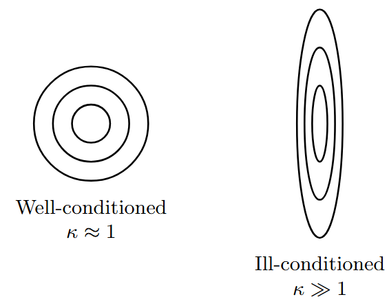
Condition Number and Convergence

Condition Number

For a quadratic function \(f(x) = \frac{1}{2}x^T A x\):

\[\kappa(A) = \frac{\lambda_{\max}(A)}{\lambda_{\min}(A)}\]

Impact on Optimization:

\(\kappa \approx 1\): Well-conditioned, fast convergence
\(\kappa \gg 1\): Ill-conditioned, slow convergence
Affects choice of optimization method

well-conditioned (circular) and ill-conditioned (elliptical) contours

Classification of Optimization Methods

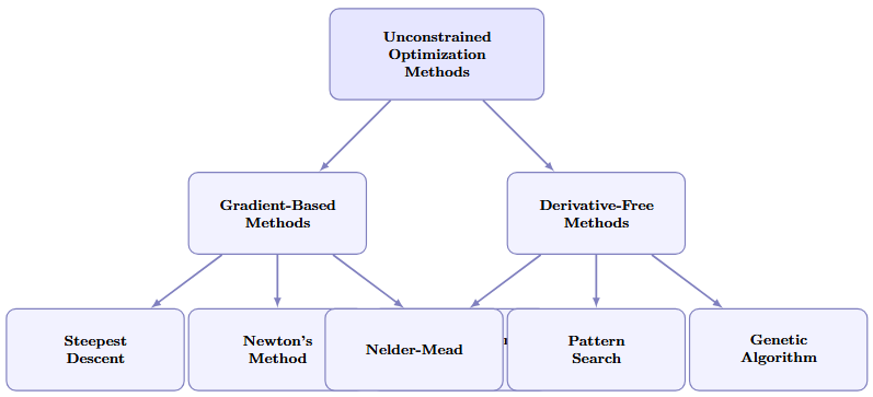
Gradient-Based Methods

General Framework: \(x_{k+1} = x_k + \alpha_k d_k\)

Steepest Descent: \(d_k = -\nabla f(x_k)\)
- Simple implementation
- Guaranteed descent direction
- Slow convergence for ill-conditioned problems
Newton’s Method: \(d_k = -[\nabla^2 f(x_k)]^{-1} \nabla f(x_k)\)
- Quadratic convergence near solution
- Requires Hessian computation and inversion
- May not converge if Hessian is not positive definite
Quasi-Newton (BFGS): Approximates Hessian inverse
- Superlinear convergence
- Lower computational cost than Newton’s method
- Robust for engineering applications

Method Comparison and Selection Criteria

Method	Derivatives	Convergence	Robustness	Cost/Iteration
Steepest Descent	\(\nabla f\)	Linear	High	Low
Conjugate Gradient	\(\nabla f\)	Superlinear	Medium	Low
Newton’s Method	\(\nabla f, \nabla^2 f\)	Quadratic	Low	High
Quasi-Newton (BFGS)	\(\nabla f\)	Superlinear	High	Medium
Trust Region	\(\nabla f, \nabla^2 f\)	Robust	Very High	High
Nelder-Mead	None	Slow	Medium	Low

Selection Guidelines:

Smooth, well-conditioned: Newton’s method
General engineering problems: BFGS
Large-scale problems: Conjugate gradient
Noisy/discontinuous: Derivative-free methods

Implementation Challenges

Initial Guess Selection:
- Critical for convergence to good local minimum
- Use engineering insight or multiple starting points
- Consider bounds on physical variables
Convergence Criteria:
- Gradient norm: \(\|\nabla f(x_k)\| < \epsilon_g\)
- Function change: \(|f(x_{k+1}) - f(x_k)| < \epsilon_f\)
- Step size: \(\|x_{k+1} - x_k\| < \epsilon_x\)
Numerical Issues:
- Finite precision arithmetic
- Gradient approximation errors
- Matrix conditioning problems
Scaling and Preconditioning:
- Normalize variables to similar scales
- Use physical units appropriately
- Precondition ill-conditioned problems

Summary

Key Takeaways:

Unconstrained nonlinear optimization is fundamental to engineering design and analysis
Nonlinearity introduces challenges: multiple optima, ill-conditioning, dimensionality
Objective function properties (convexity, smoothness, conditioning) guide method selection
Gradient-based methods offer fast convergence but require derivatives
Derivative-free methods handle noisy or discontinuous functions
Practical implementation requires careful attention to initialization and convergence

Next Lectures

Line Search Methods and Step Size Selection
Gradient-Based Algorithms: Steepest Descent and Conjugate Gradient
Newton and Quasi-Newton Methods
Trust Region Methods