Introduction to the Two-Phase Method
Definition
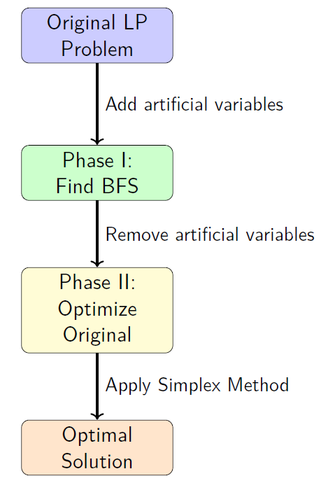
The Two-Phase Method is a systematic technique for solving linear programming problems when an obvious initial basic feasible solution (BFS) is not available.
Two Phases:
-
Phase I: Find any basic feasible solution by solving an auxiliary problem
-
Phase II: Optimize the original objective function starting from the BFS found in Phase I
Key Insight
We solve a simpler problem first to get started, then solve the actual problem we care about.
When Do We Need the Two-Phase Method?
The Challenge
The Simplex Method requires an initial basic feasible solution, but this isn’t always obvious.
Problematic Situations:
-
Constraints with \(\geq\) inequalities (no natural slack variables)
-
Equality constraints (no slack variables at all)
-
Negative right-hand side values
-
Mixed constraint types making initialization complex
Example
In \(x_1 + x_2 \geq 4\), setting \(x_1 = x_2 = 0\) violates the constraint, so we can’t start with the origin.
Mathematical Foundation
Standard Form Requirements
Every LP problem must be in standard form for simplex method:
Conversion Rules:
-
\(\leq\) constraints: Add slack variables \(s_i \geq 0\)
-
\(\geq\) constraints: Subtract surplus variables \(s_i \geq 0\), then add artificial variables
-
\(=\) constraints: Add artificial variables directly
-
Negative RHS: Multiply constraint by \(-1\) and flip inequality
Key Issue
After conversion, we may lack \(m\) obvious basic variables for \(m\) constraints.
Two-Phase Method Overview
Phase I: Finding a Basic Feasible Solution
-
Goal: Create an easy-to-solve problem whose solution gives us a starting point.
-
Method: Add artificial variables to create an obvious starting solution.
Transformation
Original Problem:
Auxiliary Problem (Phase I):
where \(\mathbf{w} = (w_1, w_2, \ldots, w_m)^T\) are artificial variables.
Theoretical Basis of Phase I
Why This Works
-
Artificial variables \(w_i\) provide immediate basic variables
-
Initial BFS: \(\mathbf{x} = \mathbf{0}\), \(\mathbf{w} = \mathbf{b}\)
-
If \(\min \sum w_i = 0\), then \(w_i = 0\) for all \(i\) (since \(w_i \geq 0\))
-
When \(\mathbf{w} = \mathbf{0}\), we have \(\mathbf{A}\mathbf{x} = \mathbf{b}\) with \(\mathbf{x} \geq \mathbf{0}\)
Critical Insight
The auxiliary problem is always feasible because we can set \(\mathbf{w} = \mathbf{b} \geq \mathbf{0}\).
Feasibility Test
-
If \(\min \sum w_i = 0\): Original problem is feasible
-
If \(\min \sum w_i > 0\): Original problem is infeasible
Phase I: Algorithm Steps
Phase I Algorithm
- Convert the original LP to standard form (all constraints as equalities).
- Add artificial variables wi to constraints that lack basic variables.
- Set up auxiliary problem: \( \text{minimize}~ \sum_{i=1}^{m} w_i \)
- Create initial tableau with artificial variables as basic variables.
- Apply Simplex Method to the auxiliary problem.
- If Optimal value > 0, then STOP: Original problem is infeasible.
-
Else if Optimal value = 0, then BFS found for original problem.
- If some artificial variables are basic with value 0, remove corresponding redundant constraints.
- Remove artificial variables and proceed to Phase II.
Phase I: Setting Up the Initial Tableau
-
Artificial variables start as basic variables with value equal to RHS
-
Original variables start as non-basic (value = 0)
-
Objective row coefficients ensure we’re minimizing \(\sum w_i\)
| Basic | \(x_1\) | \(x_2\) | \(\cdots\) | \(x_n\) | \(w_1\) | \(w_2\) | \(\cdots\) | \(w_m\) | RHS |
|---|---|---|---|---|---|---|---|---|---|
| \(w_1\) | \(a_{11}\) | \(a_{12}\) | \(\cdots\) | \(a_{1n}\) | 1 | 0 | \(\cdots\) | 0 | \(b_1\) |
| \(w_2\) | \(a_{21}\) | \(a_{22}\) | \(\cdots\) | \(a_{2n}\) | 0 | 1 | \(\cdots\) | 0 | \(b_2\) |
| \(\vdots\) | \(\vdots\) | \(\vdots\) | \(\ddots\) | \(\vdots\) | \(\vdots\) | \(\vdots\) | \(\ddots\) | \(\vdots\) | \(\vdots\) |
| \(w_m\) | \(a_{m1}\) | \(a_{m2}\) | \(\cdots\) | \(a_{mn}\) | 0 | 0 | \(\cdots\) | 1 | \(b_m\) |
| \(z\) | \(-\sum_{i=1}^{m} a_{i1}\) | \(-\sum_{i=1}^{m} a_{i2}\) | \(\cdots\) | \(-\sum_{i=1}^{m} a_{in}\) | 0 | 0 | \(\cdots\) | 0 | \(-\sum_{i=1}^{m} b_i\) |
Note: Objective row coefficients are calculated to eliminate artificial variables from the objective function.
Handling Different Constraint Types
Constraint Type Analysis
-
\(\leq\) constraints: Add slack variable \(s \geq 0\). No artificial variable needed.
-
\(\geq\) constraints: Subtract surplus \(s \geq 0\), add artificial \(w \geq 0\).
-
\(=\) constraints: Add artificial variable \(w \geq 0\) directly.
-
Negative RHS: Multiply by \(-1\), then apply above rules.
Example Transformations:
Special Case: Basic Artificial Variables with Zero Value
-
Situation: After Phase I, some artificial variables remain basic with value 0.
-
Implications:
-
The corresponding constraints may be redundant
-
Need to remove artificial variables from basis before Phase II
-
-
Solution Methods:
-
Pivot Operation: Find non-zero element in artificial variable’s row
-
Row Elimination: If entire row is zero, constraint is redundant
-
Basis Exchange: Replace artificial variable with regular variable
-
Critical Rule
Never proceed to Phase II with artificial variables in the basis.
Phase II: Optimizing the Original Objective
-
Goal Optimize the original objective function starting from the BFS found in Phase I.
-
Steps:
-
Remove all artificial variable columns from the tableau
-
Replace the objective row with original objective coefficients
-
Adjust objective row coefficients for basic variables
-
Apply Simplex Method until optimality
-
Critical Check
If any artificial variable is basic with a positive value after Phase I, the original problem is infeasible.
Why This Works
Phase I guarantees \(\sum w_i = 0\), meaning each \(w_i = 0\), so we have a feasible solution to the original problem.
Phase II: Objective Row Adjustment
-
Problem: Original objective coefficients may violate optimality conditions.
-
Solution: Adjust coefficients using basic variable relationships.
Adjustment Formula
For each non-basic variable \(x_j\):
where:
-
\(\bar{c}_j\): Adjusted coefficient for variable \(x_j\)
-
\(c_j\): Original objective coefficient for \(x_j\)
-
\(c_i\): Original objective coefficient for basic variable in row \(i\)
-
\(a_{ij}\): Tableau coefficient in row \(i\), column \(j\)
Adjusted objective value: \(\bar{z} = \sum_{i \in \text{Basic}} c_i \cdot b_i\)
Detecting Unbounded Solutions
-
Phase I completes successfully (problem is feasible)
-
During Phase II, entering variable has no positive ratios
When does unboundedness occur?
Detection Criteria:
Unbounded Test
If entering variable \(x_j\) has coefficient \(c_j < 0\) but all \(a_{ij} \leq 0\) for \(i = 1, 2, \ldots, m\), then the problem is unbounded.
Interpretation:
-
Variable \(x_j\) can increase indefinitely
-
Objective function can decrease without bound (for minimization)
-
Problem has no finite optimal solution
Detecting Multiple Optimal Solutions
Condition: Multiple optimal solutions exist when the final optimal tableau has zero coefficients for non-basic variables.
Detection Method:
-
Complete Phase II optimization
-
Check objective row coefficients for non-basic variables
-
If any coefficient equals zero, multiple solutions exist
Finding Alternative Solutions:
-
Identify non-basic variable with zero coefficient
-
Pivot on that variable (choose any positive ratio)
-
New basic solution is also optimal
Practical Significance
Multiple optimal solutions provide flexibility in implementation and can account for additional criteria not captured in the original model.
Degeneracy and Cycling
Degeneracy Issues
Definition: A basic feasible solution is degenerate if one or more basic variables equal zero.
Implications:
-
May cause cycling in simplex method
-
Ratio test may have ties
-
Objective value may not improve in some iterations
Anti-Cycling Rules
-
Bland’s Rule: Choose smallest index variable to enter/leave
-
Lexicographic Rule: Use lexicographic ordering for tie-breaking
-
Random Perturbation: Add small random values to break ties
Practical Note: Modern LP solvers automatically handle degeneracy.
Detailed Example
Problem:
Step 1: Convert to Standard Form Introduce surplus variables \(s_1, s_2 \geq 0\):
Problem: No obvious basic variables! We need artificial variables.
Example: Feasible Region Visualization
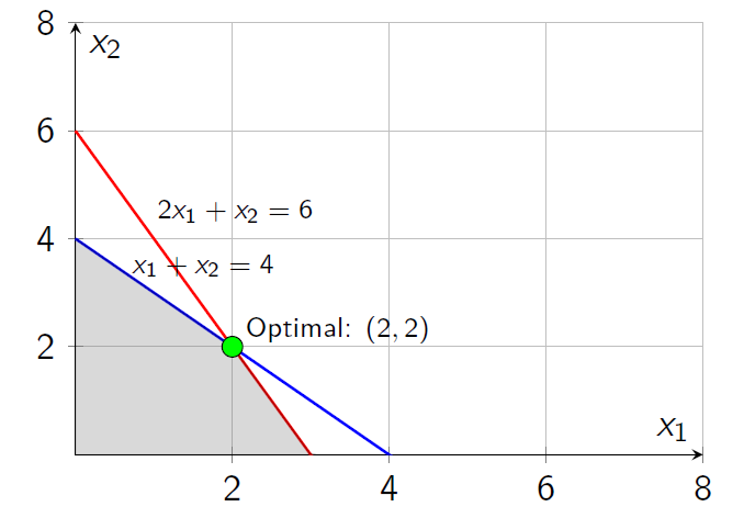
Note: Feasible region is above/right of both constraint lines. Origin \((0,0)\) is infeasible.
Example: Phase I Setup
Add Artificial Variables: \(w_1, w_2 \geq 0\)
Initial Basic Solution: \(w_1 = 4, w_2 = 6\), all others = 0
Initial Tableau:
| Basic | \(x_1\) | \(x_2\) | \(s_1\) | \(s_2\) | \(w_1\) | \(w_2\) | RHS |
|---|---|---|---|---|---|---|---|
| \(w_1\) | 1 | 1 | -1 | 0 | 1 | 0 | 4 |
| \(w_2\) | 2 | 1 | 0 | -1 | 0 | 1 | 6 |
| \(z\) | -3 | -2 | 1 | 1 | 0 | 0 | -10 |
Calculation: \(z\)-row coefficients ensure \(z = w_1 + w_2 = 10\) initially.
Example: Phase I - Iteration 1
Pivot Selection: Most negative coefficient is \(-3\) (column \(x_1\)).
Ratio Test: \(\min\{4/1, 6/2\} = \min\{4, 3\} = 3\) (row 2).
Pivot Element: Row 2, Column \(x_1\) (value = 2).
After Pivoting:
| Basic | \(x_1\) | \(x_2\) | \(s_1\) | \(s_2\) | \(w_1\) | \(w_2\) | RHS |
|---|---|---|---|---|---|---|---|
| \(w_1\) | 0 | 0.5 | -1 | 0.5 | 1 | -0.5 | 1 |
| \(x_1\) | 1 | 0.5 | 0 | -0.5 | 0 | 0.5 | 3 |
| \(z\) | 0 | -0.5 | 1 | -0.5 | 0 | 1.5 | -1 |
Current Solution: \(x_1 = 3, w_1 = 1\), others = 0. Objective = 1.
Example: Phase I - Iteration 2
Pivot Selection: Most negative coefficient is -0.5 (column \(x_2\)).
Ratio Test: \(\min\{1/0.5, 3/0.5\} = \min\{2, 6\} = 2\) (row 1).
Pivot Element: Row 1, Column \(x_2\) (value = 0.5).
After Pivoting:
| Basic | \(x_1\) | \(x_2\) | \(s_1\) | \(s_2\) | RHS |
|---|---|---|---|---|---|
| \(x_2\) | 0 | 1 | -2 | 1 | 2 |
| \(x_1\) | 1 | 0 | 1 | -1 | 2 |
| \(z\) | 0 | 0 | 0 | 0 | 0 |
Phase I Complete: Optimal value = 0, BFS found: \(x_1 = 2, x_2 = 2\).
Example: Phase II Setup
Starting Point: \( x_1 = 2, x_2 = 2, s_1 = 0, s_2 = 0 \)
Original Objective: Minimize \(2x_1 + 3x_2\)
Phase II Initial Tableau:
| Basic | \(x_1\) | \(x_2\) | \(s_1\) | \(s_2\) | RHS |
|---|---|---|---|---|---|
| \(x_2\) | 0 | 1 | -2 | 1 | 2 |
| \(x_1\) | 1 | 0 | 1 | -1 | 2 |
| \(z\) | 2 | 3 | 0 | 0 | 0 |
Adjustment Needed: Basic variables \(x_1\) and \(x_2\) have non-zero coefficients in objective row.
Corrections:
-
\(\bar{c}_{s_1} = 0 - 2(1) - 3(-2) = 4\)
-
\(\bar{c}_{s_2} = 0 - 2(-1) - 3(1) = -1\)
-
\(\bar{z} = 2(2) + 3(2) = 10\)
Example: Phase II - Corrected Tableau
Corrected Phase II Tableau:
| Basic | \(x_1\) | \(x_2\) | \(s_1\) | \(s_2\) | RHS |
|---|---|---|---|---|---|
| \(x_2\) | 0 | 1 | -2 | 1 | 2 |
| \(x_1\) | 1 | 0 | 1 | -1 | 2 |
| \(z\) | 0 | 0 | 4 | -1 | 10 |
Optimality Check: Coefficient of \(s_2\) is negative (-1), so not optimal yet.
Pivot Selection: Enter \(s_2\) (most negative coefficient).
Ratio Test: \(\min\{2/1, \text{undefined}\} = 2\) (row 1, since \(-1 < 0\)).
Pivot Element: Row 1, Column \(s_2\) (value = 1).
Example: Phase II - Final Iteration
After Pivoting:
| Basic | \(x_1\) | \(x_2\) | \(s_1\) | \(s_2\) | RHS |
|---|---|---|---|---|---|
| \(s_2\) | 0 | 1 | -2 | 1 | 2 |
| \(x_1\) | 1 | 1 | -1 | 0 | 4 |
| \(z\) | 0 | 1 | 2 | 0 | 12 |
Optimality Check: All coefficients in objective row are non-negative.
Optimal Solution:
-
\(x_1 = 4, x_2 = 0\)
-
Minimum objective value = 12
Verification
Check constraints: \(4 + 0 = 4 \geq 4\) \(\checkmark\), \(2(4) + 0 = 8 \geq 6\) \(\checkmark\)
Summary and Key Takeaways
Two-Phase Method Algorithm
Phase I:
-
Add artificial variables to create initial BFS
-
Solve auxiliary problem: minimize \(\sum w_i\)
-
If optimal value \(> 0\), original problem is infeasible
-
If optimal value \(= 0\), proceed to Phase II
Phase II:
-
Remove artificial variables from tableau
-
Replace objective function with original
-
Adjust objective coefficients for basic variables
-
Apply simplex method until optimality
Computational Complexity
Complexity Analysis
-
Phase I: At most \(\binom{m+n}{m}\) iterations (same as standard simplex)
-
Phase II: At most \(\binom{m+n}{m}\) iterations
-
Total: \(O(2^{\min(m,n)})\) worst-case, polynomial average-case
-
Space: \(O(mn)\) for tableau storage
Practical Performance:
-
Most problems solve in \(O(m)\) to \(O(n)\) iterations
-
Phase I typically requires fewer iterations than Phase II
-
Modern implementations use revised simplex for efficiency
When to Use Two-Phase Method
Recommended Scenarios
-
Problems with \(\geq\) or \(=\) constraints
-
Mixed constraint types
-
When Big-M method is numerically unstable
-
Academic/educational contexts for clarity
Alternative Methods
-
Big-M Method: Simpler setup, potential numerical issues
-
Dual Simplex: Efficient for certain problem structures
-
Interior Point: Better for very large problems
Best Practice
Use Two-Phase Method when numerical accuracy is critical or when learning simplex fundamentals.
Common Pitfalls and Troubleshooting
Frequent Mistakes:
-
Forgetting to remove artificial variables before Phase II
-
Incorrect objective row adjustments in Phase II
-
Missing degeneracy checks
-
Improper handling of basic artificial variables with zero value
Debugging Tips:
-
Always verify constraint satisfaction
-
Check that \(\sum w_i = 0\) at end of Phase I
-
Ensure no artificial variables remain basic in Phase II
-
Validate optimality conditions before declaring solution
Memory Aid
"Phase I finds feasibility, Phase II finds optimality"
Extensions and Advanced Topics
Advanced Considerations
-
Sensitivity Analysis: How solution changes with parameter variations
-
Parametric Programming: Systematic parameter variation studies
-
Integer Programming: Two-phase method as LP relaxation
-
Network Flows: Specialized two-phase algorithms
Research Directions:
-
Hybrid Phase I/Phase II algorithms
-
Parallel implementations
-
Machine learning-guided pivot selection
-
Quantum computing adaptations
References and Further Reading
Essential Textbooks:
-
Hillier & Lieberman: Introduction to Operations Research
-
Bazaraa, Jarvis & Sherali: Linear Programming and Network Flows
-
Chvátal: Linear Programming
Software Implementations:
-
CPLEX, Gurobi, GLPK
-
Python: SciPy, PuLP, CVXPY
-
R: lpSolve, Rglpk
-
MATLAB: Optimization Toolbox
Online Resources:
-
MIT OpenCourseWare: Linear Programming
-
Stanford CS261: Optimization
-
NEOS Optimization Server