Trust Region Methods: Optimization Techniques

Trust Region Framework

Alternative to line search methods for nonlinear optimization
Basic idea: Approximate the objective function in a neighborhood (trust region)
At each iteration:
- Build a local model (usually quadratic) within trust region radius \(\Delta_k\)
- Solve constrained subproblem to find step within trust region
- Evaluate actual vs. predicted improvement
- Adjust trust region radius based on performance
Particularly effective for non-convex problems

Key Components

Local model (typically quadratic approximation)
Trust region radius \(\Delta_k\)
Acceptance/rejection criteria
Radius adjustment strategy

Trust Region vs Line Search

Line Search:

Fix direction, choose step length
\(x_{k+1} = x_k + \alpha_k p_k\)
May fail for indefinite Hessians
Can take inefficient zigzag paths

Trust Region:

Fix step length, choose direction
\(x_{k+1} = x_k + p_k\) with \(\|p_k\| \leq \Delta_k\)
Handles indefinite Hessians naturally
Adapts both direction and magnitude

When to Use Trust Region

Non-convex optimization problems
Noisy or discontinuous derivatives
Problems where Newton’s method struggles

Mathematical Formulation

Original problem:

\[\min_{x \in \mathbb{R}^n} f(x)\]
Trust region subproblem:

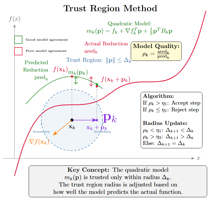
\[\min_p m_k(p) = f_k + \nabla f_k^T p + \frac{1}{2}p^T B_k p\]

\[\text{subject to } \|p\| \leq \Delta_k\]

where:
- \(f_k = f(x_k)\), \(\nabla f_k = \nabla f(x_k)\)
- \(B_k\) is Hessian or approximation
- \(\Delta_k\) is trust region radius
- \(\|\cdot\|\) is typically \(\ell_2\) norm

Basic Trust Region Algorithm

Algorithm: Trust Region Method

Initialize \( x_0 \), \( \Delta_0 > 0 \), \( 0 < \eta_1 < \eta_2 < 1 \)
For \( k = 0, 1, 2, \ldots \):
1. Solve trust region subproblem to get \( p_k \)
2. Compute actual reduction: \( \text{ared}_k = f(x_k) - f(x_k + p_k) \)
3. Compute predicted reduction: \( \text{pred}_k = m_k(0) - m_k(p_k) \)
4. Compute ratio: \( \rho_k = \frac{\text{ared}_k}{\text{pred}_k} \)
5. If \( \rho_k > \eta_1 \):
  - \( x_{k+1} = x_k + p_k \) (Accept step)
6. Else:
  - \( x_{k+1} = x_k \) (Reject step)
7. Update trust region radius \( \Delta_{k+1} \) based on \( \rho_k \)

Solving the Trust Region Subproblem

Exact Solution (KKT Conditions)

The exact solution \(p^*\) satisfies:

\[(B_k + \lambda I)p^* = -\nabla f_k\]

with complementary slackness:

\[\lambda \geq 0, \quad \lambda(\Delta_k - \|p^*\|) = 0\]

Two cases:
- Interior solution (\(\|p^*\| < \Delta_k\)): \(\lambda = 0\), unconstrained minimizer
- Boundary solution (\(\|p^*\| = \Delta_k\)): \(\lambda > 0\), constrained
Exact solution computationally expensive for large problems
Several approximate strategies exist

Cauchy Point Method

Computes the minimizer along steepest descent direction within trust region
Step: \(p_k^{SD} = -\alpha \nabla f_k\) where \(\alpha > 0\)
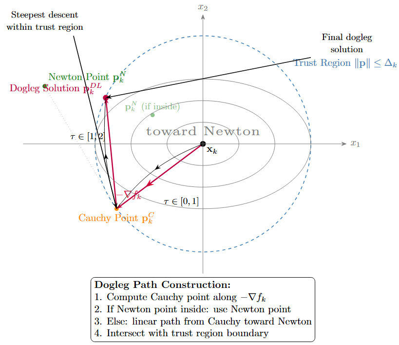
Cauchy point: \(p_k^C = -\tau_k \frac{\Delta_k}{\|\nabla f_k\|} \nabla f_k\)

where \(\tau_k = \min\left(1, \frac{\|\nabla f_k\|^3}{\Delta_k \nabla f_k^T B_k \nabla f_k}\right)\) if \(\nabla f_k^T B_k \nabla f_k > 0\)
Properties:
- Inexpensive to compute: \(O(n)\) operations
- Global convergence guaranteed
- Often used as fallback in more sophisticated methods
- Provides lower bound on improvement

Dogleg Method

Requirements: \(B_k\) positive definite

Two key points:

Cauchy point: \(p_k^C\)
Newton point: \(p_k^N = -B_k^{-1}\nabla f_k\)

Dogleg path:

If \(\|p_k^N\| \leq \Delta_k\): return \(p_k^N\)
Else: linear combination
\[p_k(\tau) = \begin{cases} \tau p_k^C & 0 \leq \tau \leq 1\\ p_k^C + (\tau-1)(p_k^N - p_k^C) & 1 \leq \tau \leq 2 \end{cases}\]

Subspace Minimization (Steihaug-Toint)

Also known as truncated conjugate gradient method
Minimizes model over Krylov subspace:
\[\mathcal{K}_j = \text{span}\{\nabla f_k, B_k\nabla f_k, \ldots, B_k^{j-1}\nabla f_k\}\]
Algorithm terminates when:
- Conjugate gradient converges
- Trust region boundary reached
- Negative curvature detected
Advantages:
- Handles indefinite \(B_k\) gracefully
- Better than dogleg for indefinite problems
- Scales well to large problems

Convergence Properties

Theorem: Global Convergence

Under standard assumptions (continuous derivatives, bounded level sets), trust region methods converge to a stationary point:

\[\lim_{k \to \infty} \|\nabla f_k\| = 0\]

Local Convergence Rates

Linear convergence: Always guaranteed
Superlinear convergence: When \(B_k \approx \nabla^2 f(x_k)\) and \(\Delta_k\) eventually inactive
Quadratic convergence: When \(B_k = \nabla^2 f(x_k)\) exactly

Key Assumption

The model \(m_k(p)\) provides sufficient decrease compared to Cauchy point

Adaptive Radius Adjustment

Critical for practical performance
Based on ratio of actual to predicted reduction:
\[\rho_k = \frac{f(x_k) - f(x_k + p_k)}{m_k(0) - m_k(p_k)} = \frac{\text{ared}_k}{\text{pred}_k}\]
Radius update rules:
- \(\rho_k < \eta_1\): Poor model, decrease radius
  \[\Delta_{k+1} = \gamma_1 \|p_k\|, \quad \gamma_1 \in (0, 1)\]
- \(\eta_1 \leq \rho_k < \eta_2\): Acceptable model, keep radius
  \[\Delta_{k+1} = \Delta_k\]
- \(\rho_k \geq \eta_2\): Good model, possibly increase radius
  \[\Delta_{k+1} = \min(\gamma_2 \Delta_k, \Delta_{\max}) \text{ if } \|p_k\| = \Delta_k\]

Typical values: \(\eta_1 = 0.25\), \(\eta_2 = 0.75\), \(\gamma_1 = 0.5\), \(\gamma_2 = 2\)

Hessian Approximation Strategies

Exact Hessian

\(B_k = \nabla^2 f(x_k)\)
Best convergence properties
Expensive to compute and store for large \(n\)

Quasi-Newton Methods

BFGS: \(B_{k+1} = B_k + \frac{y_k y_k^T}{y_k^T s_k} - \frac{B_k s_k s_k^T B_k}{s_k^T B_k s_k}\)
SR1: \(B_{k+1} = B_k + \frac{(y_k - B_k s_k)(y_k - B_k s_k)^T}{(y_k - B_k s_k)^T s_k}\)
Limited memory versions: L-BFGS, L-SR1

Other Approximations

Finite differences
Identity matrix: \(B_k = I\) (steepest descent)
Scaled identity: \(B_k = \sigma_k I\)

Practical Applications

Chemical engineering: Parameter estimation in complex reaction models
Computer vision: Bundle adjustment in 3D reconstruction
Machine learning: Training deep neural networks (alternative to Adam/SGD)
Economics: Calibration of large-scale macroeconomic models
Computational physics: Molecular geometry optimization
Structural optimization: Design of mechanical components
Data fitting: Nonlinear regression with outliers

Advantages in Practice

More robust than line search for non-convex problems
Handles indefinite Hessians gracefully
Automatic step size control via radius adjustment
Good performance even with approximate Hessians

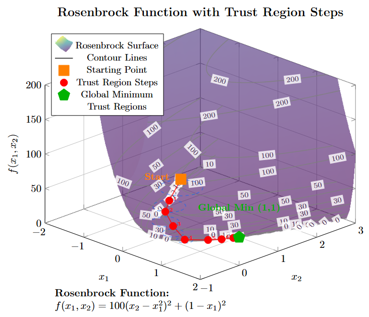
Example: Rosenbrock Function

Classic test problem:
\[f(x,y) = (a-x)^2 + b(y-x^2)^2\]
Standard values: \(a=1\), \(b=100\)
Highly nonlinear, curved valley
Challenges:
- Ill-conditioned Hessian
- Narrow curved valley
- Global minimum at \((1,1)\)
Trust region adapts step size automatically in different regions

Rosenbrock function with trust region steps

Implementation Tips

Computational Efficiency

Use matrix factorizations (Cholesky, eigenvalue decomposition)
Implement iterative methods for large-scale problems
Consider limited-memory quasi-Newton methods

Numerical Stability

Handle near-singular systems carefully
Use regularization when \(B_k\) is indefinite
Monitor condition numbers

Parameter Tuning

Initial trust region radius: \(\Delta_0 = 0.1 \cdot \|x_0\|\) or \(\Delta_0 = 1\)
Conservative radius updates for noisy functions
Problem-specific termination criteria

Summary

Trust region methods provide robust optimization framework
Key features:
- Local model constrained to trust region
- Adaptive radius control based on model quality
- Global convergence guarantees
- Handle indefinite Hessians naturally
Solution strategies range from simple (Cauchy point) to sophisticated (Steihaug-Toint)
Particularly valuable for:
- Non-convex problems
- Problems with indefinite Hessians
- Cases where line search struggles
- Noisy objective functions

Future Directions

Adaptive model selection
Trust region methods for constrained optimization
Stochastic trust region methods

Trust Region Methods

Introduction