What is Optimization?
The process of finding the best solution from a set of available alternatives according to some criterion.
Everyday Examples
-
Finding the shortest route to work
-
Maximizing profit while minimizing cost
-
Training a neural network (minimizing loss)
-
Portfolio optimization in finance
Key Question
What makes a problem nonlinear?
General Optimization Problem Formulation
Standard Form
-
\(x = (x_1, x_2, \ldots, x_n)^T\): Decision variables
-
\(f(x): \mathbb{R}^n \to \mathbb{R}\): Objective function
-
\(g_i(x) \leq 0\): Inequality constraints
-
\(h_j(x) = 0\): Equality constraints
-
\(\mathcal{X}\): Feasible region/domain
Terminology
Key Definitions
-
Feasible point: \(x\) satisfying all constraints
-
Feasible set: \(\mathcal{F} = \{x : g_i(x) \leq 0, h_j(x) = 0, x \in \mathcal{X}\}\)
-
Optimal solution: \(x^* \in \mathcal{F}\) such that \(f(x^*) \leq f(x)\) \(\forall x \in \mathcal{F}\)
-
Optimal value: \(f^* = f(x^*)\)
Simple Example
Linear vs. Nonlinear Optimization
Linear Program
-
Objective function is linear
-
All constraints are linear
-
Feasible region is a polyhedron
-
Global optimum always exists (if bounded)
-
Polynomial-time solvable (Simplex, Interior Point)
Nonlinear Programming (NLP)
Nonlinear Program
At least one of \(f(x)\), \(g_i(x)\), or \(h_j(x)\) is nonlinear
| Aspect | Linear | Nonlinear |
|---|---|---|
| Objective | \(c^T x\) | \(x^2 + \sin(x)\) |
| Constraints | \(Ax \leq b\) | \(x_1^2 + x_2^2 \leq 1\) |
| Feasible region | Polyhedron | Curved boundaries |
| Optima | Single global | Multiple local |
| Complexity | Polynomial | Generally NP-hard |
| Algorithms | Simplex, IPM | Gradient-based |
Why Nonlinear Optimization is Challenging
-
Multiple local optima
-
No polynomial-time guarantee
-
Sensitivity to starting point
-
Convergence issues
-
Constraint qualification
Types of Nonlinear Problems
By Constraints
-
Unconstrained: \(\min f(x)\)
-
Equality constrained: \(\min f(x)\) s.t. \(h(x) = 0\)
-
Inequality constrained: \(\min f(x)\) s.t. \(g(x) \leq 0\)
-
Mixed: Both equality and inequality constraints
By Function Properties
-
Smooth: \(f, g, h\) are continuously differentiable
-
Nonsmooth: Contains non-differentiable points
-
Convex: Special structure (global optimum guaranteed)
-
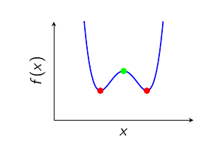
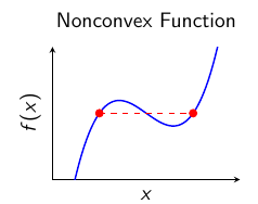
Nonconvex: General case (local optima possible)
Convexity - A Crucial Concept
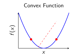
A set \(S\) is convex if for any \(x, y \in S\) and \(\lambda \in [0,1]\):
\(f\) is convex if for any \(x, y \in \text{dom}(f)\) and \(\lambda \in [0,1]\):
Golden Rule
Convex problem = Convex objective + Convex feasible set
\(\Rightarrow\) Every local minimum is a global minimum!
Visual Understanding of Convexity
Applications of Nonlinear Optimization
Engineering & Design
-
Structural optimization
-
Control system design
-
Signal processing
-
Robotics path planning
Machine Learning & AI
-
Neural network training
-
Support vector machines
-
Reinforcement learning
-
Computer vision
Economics & Finance
-
Portfolio optimization
-
Risk management
-
Option pricing
-
Resource allocation
Operations Research
-
Supply chain optimization
-
Facility location
-
Energy systems
-
Telecommunications
Case Study: Portfolio Optimization
Markowitz Mean-Variance Model
-
\(w\): Portfolio weights
-
\(\Sigma\): Covariance matrix (risk)
-
\(\mu\): Expected returns
-
\(r_{\min}\): Minimum required return
Why nonlinear? Quadratic objective function!
Solution Approaches - Preview
Analytical Approaches
-
Optimality conditions (KKT conditions)
-
Lagrange multipliers
-
Convex analysis
Numerical Methods
-
Gradient-based: Steepest descent, Newton’s method
-
Constrained: Sequential quadratic programming
-
Global: Genetic algorithms, simulated annealing
-
Modern: Interior point methods, trust region
Historical Perspective
-
1600s-1700s: Newton, Leibniz, Euler (calculus of variations)
-
1800s: Lagrange multipliers, method of Lagrange
-
1939: Karush develops optimality conditions
-
1947: Dantzig invents Simplex method (Linear Programming)
-
1951: Kuhn-Tucker extend Karush conditions (KKT)
-
1960s-1980s: Development of nonlinear programming algorithms
-
1990s-Present: Interior point methods, convex optimization
-
2000s-Present: Large-scale optimization, machine learning applications
Practical Considerations
Key Challenges in Practice
-
Scaling: How to handle large-scale problems?
-
Initialization: Where to start the algorithm?
-
Convergence: When to stop?
-
Globalization: How to avoid local optima?
-
Numerical stability: Dealing with ill-conditioning
Success Factors
-
Understanding problem structure
-
Choosing appropriate algorithms
-
Proper implementation and tuning
Summary
-
Nonlinear optimization is everywhere in science and engineering
-
Key difference from linear: local vs global optima
-
Convexity is a game-changer when present
-
Multiple solution approaches exist
-
Rich mathematical theory supports practical algorithms
Next: Mathematical Foundations & Convex Analysis