Review of Multivariable Calculus
Key Objects in Optimization
For a function \(f: \mathbb{R}^n \to \mathbb{R}\):
-
Partial derivative: \(\frac{\partial f}{\partial x_i}\) - rate of change w.r.t. \(x_i\)
-
Gradient: \(\nabla f(x) = \left[\frac{\partial f}{\partial x_1}, \dots, \frac{\partial f}{\partial x_n}\right]^T\)
-
Hessian: \(\nabla^2 f(x)_{ij} = \frac{\partial^2 f}{\partial x_i \partial x_j}\)
Example
For \(f(x,y) = x^2 + 2xy + y^3\):
Partial Derivatives - Geometric Interpretation
-
\(\frac{\partial f}{\partial x_i}\) measures rate of change along \(x_i\)-axis
-
Keep all other variables constant
-
Slope of tangent line to curve \(f(x_1, \ldots, x_i, \ldots, x_n)\)

Chain Rule (Multivariate)
If \(f(x(t), y(t))\), then:
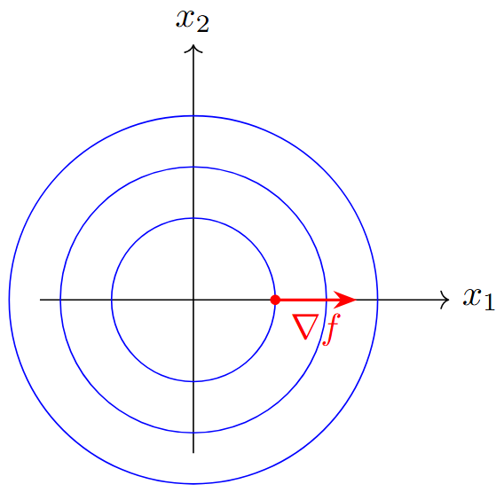
Gradients, Hessians & Jacobians
-
Points in direction of maximum increase of \(f\)
-
Orthogonal to level sets (\(\nabla f \perp \{x \mid f(x)=c\}\))
-
Critical point: \(\nabla f(x^*) = 0\)
-
Magnitude: \(\|\nabla f(x)\|\) = maximum directional derivative
Directional Derivative
Along unit vector \(d\):
Hessian Matrix: Second-Order Information
Definition
-
Symmetric (if \(f \in C^2\)): \(\frac{\partial^2 f}{\partial x_i \partial x_j} = \frac{\partial^2 f}{\partial x_j \partial x_i}\)
-
Determines curvature of \(f\)
-
Used in optimality conditions and Newton’s method
Jacobian: Vector-Valued Functions
For \(F: \mathbb{R}^n \to \mathbb{R}^m\) with \(F(x) = [F_1(x), F_2(x), \ldots, F_m(x)]^T\):
Example
Note: When \(m=1\), \(J_F = \nabla F^T\)
Taylor Series Approximations
Theorem: First-Order Approximation
For \(f \in C^1\):
Theorem : Second-Order Approximation
For \(f \in C^2\):
Error Analysis
-
First-order error: \(O(\|\Delta x\|^2)\)
-
Second-order error: \(O(\|\Delta x\|^3)\)
Why Taylor Series Matter in Optimization
Algorithm Design Foundation
-
Gradient descent: Uses 1st-order approximation
-
Newton’s method: Uses 2nd-order approximation
-
Quasi-Newton methods: Approximate 2nd-order info
Example: Quadratic Model
At each iteration, approximate \(f\) by quadratic:
Local vs. Global Behavior
Taylor approximations are local - accuracy decreases with distance from expansion point
Convex Analysis
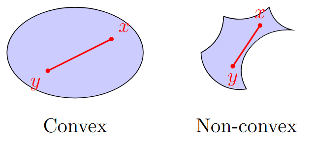
Definition : Convex Set
A set \(S \subseteq \mathbb{R}^n\) is convex if:
Examples of Convex Sets
-
Hyperplanes: \(\{x \mid a^T x = b\}\)
-
Half-spaces: \(\{x \mid a^T x \leq b\}\)
-
Balls: \(\{x \mid \|x - c\| \leq r\}\)
-
Intersection of convex sets is convex
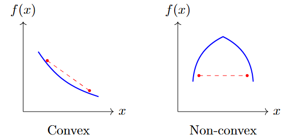
Convex Functions
A function \(f: S \to \mathbb{R}\) on convex set \(S\) is convex if:
Strictly Convex
If inequality is strict for \(x \neq y\) and \(\lambda \in (0,1)\)
Characterizations of Convex Functions
First-Order Condition
For \(f \in C^1\) on convex set \(S\), \(f\) is convex iff:
Theorem (Second-Order Condition)
For \(f \in C^2\) on convex set \(S\), \(f\) is convex iff:
(Hessian is positive semidefinite)
Key Insight
Convex functions have no local minima that are not global
Properties of Convex Functions
Preservation Under Operations
-
Positive combination: \(\alpha f + \beta g\) convex if \(\alpha, \beta \geq 0\)
-
Pointwise maximum: \(\max\{f_1(x), f_2(x), \ldots\}\) convex
-
Composition: \(g(f(x))\) convex if \(g\) convex increasing, \(f\) convex
Example (Common Convex Functions)
-
Linear: \(a^T x + b\)
-
Quadratic: \(\frac{1}{2}x^T Q x + q^T x + r\) (if \(Q \succeq 0\))
-
Exponential: \(e^{ax}\)
-
Norms: \(\|x\|_p\) for \(p \geq 1\)
-
Logarithmic barrier: \(-\sum_{i=1}^n \log(x_i)\) on \(\{x \mid x > 0\}\)
Optimality Conditions
Problem
Theorem (First-Order Necessary Condition (FONC))
If \(x^*\) is a local minimum and \(f \in C^1\), then:
Theorem (Second-Order Necessary Condition (SONC))
If \(x^*\) is a local minimum and \(f \in C^2\), then:
Critical Points
Points where \(\nabla f(x) = 0\) - could be minima, maxima, or saddle points
Sufficient Conditions
Theorem: (Second-Order Sufficient Condition (SOSC))
If \(\nabla f(x^*) = 0\) and \(\nabla^2 f(x^*) \succ 0\), then \(x^*\) is a strict local minimum.
Classification of Critical Points
-
\(\nabla^2 f \succ 0\): Local minimum
-
\(\nabla^2 f \prec 0\): Local maximum
-
\(\nabla^2 f\) indefinite: Saddle point
-
\(\nabla^2 f\) singular: Inconclusive
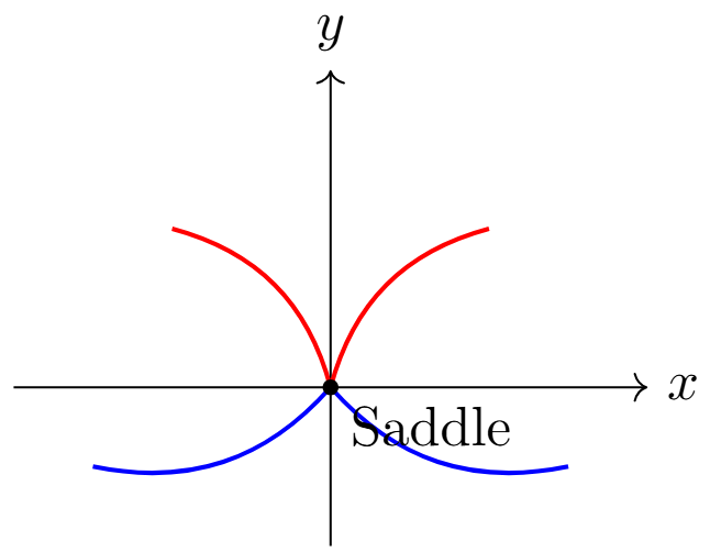
Example
For \(f(x,y) = x^2 - y^2\): \(\nabla f = [2x, -2y]^T\), \(\nabla^2 f = \begin{bmatrix} 2 & 0 \\ 0 & -2 \end{bmatrix}\)
At \((0,0)\): \(\nabla f = 0\), but \(\nabla^2 f\) is indefinite \(\Rightarrow\) saddle point
Necessary vs. Sufficient Conditions
Necessary Conditions
-
Must hold at optimum
-
Help find candidates
-
Not sufficient for optimality
Example
\(f(x) = x^4\) at \(x=0\):
-
\(f'(0) = 0\) \(\checkmark\)
-
\(f''(0) = 0\) (inconclusive)
-
But \(x=0\) is global minimum!
Sufficient Conditions
-
Guarantee optimality
-
Help verify candidates
-
Often stronger than necessary
Gap Between Necessary and Sufficient
There exist points satisfying necessary conditions but not sufficient conditions that are still optimal.
Introduction to Lagrange Multipliers
Problem (Equality Constrained Problem)
Key Insight
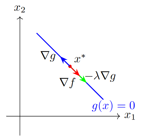
At optimum, gradient of objective must be orthogonal to feasible directions

At optimum \(x^*\):
-
\(\nabla f(x^*)\) parallel to \(\nabla g(x^*)\)
-
Both orthogonal to constraint
-
Feasible directions have zero projection on \(\nabla f\)
Lagrange Multiplier Theorem
Theorem: First-Order Necessary Conditions
Let \(x^*\) be a local minimum of \(f(x)\) subject to \(g_i(x) = 0\), \(i = 1, \ldots, m\). If \(\nabla g_1(x^*), \ldots, \nabla g_m(x^*)\) are linearly independent, then there exist multipliers \(\lambda_1^*, \ldots, \lambda_m^*\) such that:
Lagrangian Function
KKT System
Geometric Interpretation
-
\(\lambda_i^*\) measures sensitivity of optimal value to constraint \(i\)
-
\(\lambda_i^* > 0\): constraint "pushes" solution away from unconstrained optimum
-
\(\lambda_i^* < 0\): constraint "pulls" solution toward unconstrained optimum
Economic Interpretation
\(\lambda_i^*\) = shadow price of constraint \(i\)
where \(g_i(x) = b_i\) (perturbed constraint)
Simple Example: Lagrange Multipliers
Example
Minimize \(f(x,y) = x^2 + y^2\) subject to \(g(x,y) = x + y - 1 = 0\)
Solution:
-
Form Lagrangian: \(L(x,y,\lambda) = x^2 + y^2 + \lambda(x + y - 1)\)
-
KKT conditions:
\[\begin{aligned} \frac{\partial L}{\partial x} &= 2x + \lambda = 0 \\ \frac{\partial L}{\partial y} &= 2y + \lambda = 0 \\ \frac{\partial L}{\partial \lambda} &= x + y - 1 = 0 \end{aligned}\] -
Solve: From (1) and (2): \(x = y = -\frac{\lambda}{2}\)
-
Substitute into (3): \(-\frac{\lambda}{2} - \frac{\lambda}{2} - 1 = 0 \Rightarrow \lambda = -1\)
-
Therefore: \(x^* = y^* = \frac{1}{2}\), \(f^* = \frac{1}{2}\)
Preview: Inequality Constraints
Problem (General Nonlinear Program)
Karush-Kuhn-Tucker (KKT) Conditions
At optimal point \((x^*, \lambda^*, \mu^*)\):
Next lecture: Detailed KKT analysis and constraint qualifications
Key Takeaways
-
Calculus Tools: Gradients, Hessians, Jacobians are fundamental
-
Taylor Approximations: Foundation for iterative algorithms
-
Convexity: Guarantees global optimality of local solutions
-
Optimality Conditions:
-
Necessary: Must hold at optimum (help find candidates)
-
Sufficient: Guarantee optimality (help verify candidates)
-
-
Lagrange Multipliers: Handle equality constraints elegantly
Mathematical Foundation Complete
We now have the mathematical tools to tackle general nonlinear optimization problems!
Next lecture: KKT conditions and constraint qualifications
Practice Problems
-
Compute gradient and Hessian of \(f(x,y,z) = x^2y + e^{yz} + \sin(xz)\)
-
Show that \(f(x) = \|x\|_2^2\) is convex using second-order conditions
-
Find all critical points of \(f(x,y) = x^3 - 3xy^2 + y^3\) and classify them
-
Use Lagrange multipliers to minimize \(f(x,y) = xy\) subject to \(x^2 + y^2 = 1\)
-
Prove that the intersection of two convex sets is convex