Newton’s Method - Overview

• Purpose: Find stationary points of smooth functions

• Approach: Use second-order Taylor approximation

• Key Idea: Approximate function locally by quadratic and minimize exactly

• Advantages:

  • Quadratic convergence near solution

  • Scale-invariant

  • Natural for optimization problems

• Disadvantages:

  • Requires Hessian computation

  • May not converge globally

  • Expensive per iteration

Historical Context

• Isaac Newton (1643-1727): Original method for root finding

• Joseph Raphson (1648-1715): Improved formulation

• Extension to Optimization:

  • Apply Newton-Raphson to \(\nabla f(x) = 0\)

  • Use second derivatives (Hessian matrix)

• Modern Development:

  • Convergence analysis (20th century)

  • Globalization strategies

  • Computational considerations

Taylor Series Approximation

For a twice continuously differentiable function \(f: \mathbb{R}^n \to \mathbb{R}\):

Where:

• \(\nabla f(x)\) is the gradient vector

• \(\nabla^2 f(x)\) is the Hessian matrix

• \(p\) is the step vector

Key Insight: Minimize the quadratic approximation to find the step direction.

Deriving Newton’s Step

Let \(m_k(p) = f(x_k) + \nabla f(x_k)^T p + \frac{1}{2} p^T \nabla^2 f(x_k) p\)

To minimize \(m_k(p)\), set \(\nabla_p m_k(p) = 0\):

Requirements:

• \(\nabla^2 f(x_k)\) must be invertible

• Typically assume \(\nabla^2 f(x_k) \succ 0\) (positive definite)

Newton’s Method Algorithm

Local Convergence Theory

Interpretation: Near the solution, errors square at each iteration!

Convergence Rate Comparison

Note: Newton’s method achieves superlinear convergence even when convergence conditions are relaxed.

Global Convergence Issues

Problems with Pure Newton’s Method:

• Non-convex functions: May converge to saddle points or maxima

• Indefinite Hessian: \(\nabla^2 f(x_k)\) not positive definite

• Poor starting point: May diverge or converge slowly

• Singular Hessian: \(\nabla^2 f(x_k)\) not invertible

Handling Indefinite Hessians

Problem: \(\nabla^2 f(x_k)\) may not be positive definite

Solutions:

1. Modified Newton Method:

   \[H_k + \lambda_k I \succ 0\]
   Choose \(\lambda_k\) to ensure positive definiteness

2. Eigenvalue Modification:

   \[H_k = Q \Lambda Q^T \rightarrow Q |\Lambda| Q^T\]

   Replace negative eigenvalues with their absolute values

3. Cholesky with Pivoting: Add regularization during factorization

Trade-off: Modifications may slow convergence but ensure descent direction.

Line Search Newton Method

Globalization Strategy: Combine Newton direction with line search

Benefits:

• Guarantees decrease in function value

• Global convergence under mild conditions

• Preserves quadratic convergence near solution

Computational Considerations

Cost per Iteration:

• Gradient computation: \(O(n)\) (usually)

• Hessian computation: \(O(n^2)\) storage, varies in time

• Linear system solution: \(O(n^3)\) (dense) or \(O(n^{1.5})\) (sparse)

Hessian Computation Methods:

1. Analytical: Exact but may be complex to derive

2. Finite Differences:

   \[\frac{\partial^2 f}{\partial x_i \partial x_j} \approx \frac{f(x + h e_i + h e_j) - f(x + h e_i) - f(x + h e_j) + f(x)}{h^2}\]

3. Automatic Differentiation: Efficient and exact

Linear System Solution: Use Cholesky decomposition when \(H \succ 0\)

Example 1: Quadratic Function

Consider \(f(x) = \frac{1}{2} x^T Q x - b^T x\) where \(Q \succ 0\).

• \(\nabla f(x) = Qx - b\)

• \(\nabla^2 f(x) = Q\)

Newton step: \(p_k = -Q^{-1}(Qx_k - b) = Q^{-1}b - x_k\)

Update: \(x_{k+1} = x_k + p_k = Q^{-1}b\)

This is why quadratic convergence is optimal near the solution.

Example 2: Rosenbrock Function

Minimum at \((1, 1)\) with \(f(1, 1) = 0\).

Gradient:

Hessian:

Challenge: Hessian can be indefinite far from solution, requiring modifications.

Applications

Newton’s Method is Essential in:

• Machine Learning:

  • Logistic regression (IRLS algorithm)

  • Neural network training (second-order methods)

  • Support vector machines

• Statistics:

  • Maximum likelihood estimation

  • Generalized linear models

  • Bayesian inference (MAP estimation)

• Engineering:

  • Structural optimization

  • Control system design

  • Signal processing

• Economics and Finance:

  • Portfolio optimization

  • Option pricing models

  • Equilibrium analysis

Advantages of Newton’s Method

• Quadratic Convergence: Extremely fast near solution

• Scale Invariance: Performance independent of problem scaling

• Affine Invariance: Unaffected by linear transformations

• Natural for Optimization: Derived from optimization principles

• Exact for Quadratics: Optimal for quadratic functions

• Well-Understood Theory: Extensive convergence analysis

Limitations and Disadvantages

• Computational Cost: \(O(n^3)\) per iteration

• Memory Requirements: \(O(n^2)\) for Hessian storage

• Hessian Computation: May be difficult or expensive

• Global Convergence: No guarantee without modifications

• Indefinite Hessian: Requires special handling

• Singular Points: May fail at saddle points

Important Variants

1. Damped Newton Method:

   \[x_{k+1} = x_k - \alpha_k H_k^{-1} g_k\]

   Use line search to choose \(\alpha_k\)

2. Trust Region Newton:

   \[\min_{p} \nabla f(x_k)^T p + \frac{1}{2} p^T \nabla^2 f(x_k) p\]
   subject to \(\|p\| \leq \Delta_k\)

3. Quasi-Newton Methods: Approximate Hessian with updates (BFGS, L-BFGS)

4. Gauss-Newton: For nonlinear least squares problems

5. Levenberg-Marquardt: Combines Gauss-Newton with steepest descent

Relationship to Other Methods

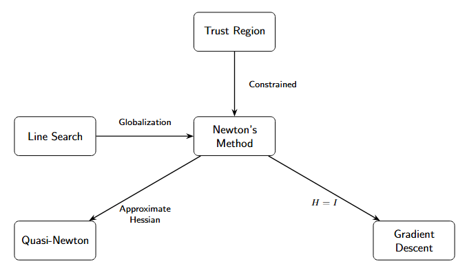
Newton’s method serves as the foundation for many advanced optimization algorithms.

Summary

Key Takeaways:

• Newton’s method uses second-order information for fast convergence

• Achieves quadratic convergence near the solution

• Requires positive definite Hessian for guaranteed descent

• Computational cost is \(O(n^3)\) per iteration

• Global convergence requires modifications (line search, trust region)

• Exact solution for quadratic functions in one step

• Foundation for many modern optimization algorithms

Further Reading

Recommended Textbooks:

• Nocedal & Wright: Numerical Optimization

• Boyd & Vandenberghe: Convex Optimization

• Bertsekas: Nonlinear Programming

Next Topics:

• Quasi-Newton Methods (BFGS, L-BFGS)

• Trust Region Methods

• Constrained Optimization (KKT conditions)

• Interior Point Methods