Introduction
- Multivariable optimization: Optimizes functions of multiple variables without constraints.
- Key tools: Gradient and Hessian provide critical information for finding extrema.
- Applications: Used in engineering, economics, and machine learning for multidimensional problems.
- Objective: This lecture covers definitions, conditions, and methods for classifying extrema.
Multivariable Optimization Concepts
Key Definitions
- Function: \( f(\mathbf{x}) \), where \( \mathbf{x} = (x_1, x_2, \ldots, x_n)^T \).
- Gradient vector: \( \nabla f = \left( \frac{\partial f}{\partial x_1}, \ldots, \frac{\partial f}{\partial x_n} \right)^T \).
- Hessian matrix: \( H(f) = \left[ \frac{\partial^2 f}{\partial x_i \partial x_j} \right]_{n \times n} \).
Theorem: Necessary Condition
If \( f(\mathbf{x}) \) has a local extremum at \( \mathbf{x}^* \) and is differentiable, then \( \nabla f(\mathbf{x}^*) = \mathbf{0} \).
Taylor Series Expansion
Second-Order Approximation
For a function \( f(\mathbf{x}) \) about point \( \mathbf{x}^* \):
\[ f(\mathbf{x}) \approx f(\mathbf{x}^*) + \nabla f(\mathbf{x}^*)^T (\mathbf{x} - \mathbf{x}^*) + \frac{1}{2} (\mathbf{x} - \mathbf{x}^*)^T H(\mathbf{x}^*) (\mathbf{x} - \mathbf{x}^*) \]
- First-order term: Gradient provides slope information.
- Second-order term: Hessian provides curvature information.
- Basis: Used in many optimization algorithms.
Hessian Analysis Methods
Theorem: Second-Order Sufficient Condition
Let \( \nabla f(\mathbf{x}^*) = \mathbf{0} \). Then:
- Positive definite Hessian: \( \mathbf{x}^* \) is a local minimum.
- Negative definite Hessian: \( \mathbf{x}^* \) is a local maximum.
- Indefinite Hessian: \( \mathbf{x}^* \) is a saddle point.
Checking Definiteness
- Eigenvalue Test:
- All \( \lambda_i > 0 \): Positive definite.
- All \( \lambda_i < 0 \): Negative definite.
- Mixed signs: Indefinite.
- Sylvester’s Criterion:
- All leading principal minors \( > 0 \): Positive definite.
- Signs alternate starting with \( < 0 \): Negative definite.
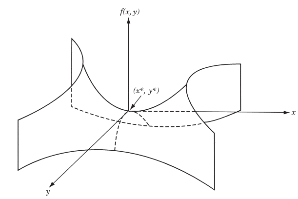
Saddle Point
- Definition: A point where the function is neither a maximum nor minimum.
- Gradient Condition: All first partial derivatives are zero.
- Surface Behavior: Curves upward in one direction, downward in another.
Example: For \( f(x, y) = x^2 - y^2 \):
- Along \( x \)-axis: \( f(x, 0) = x^2 \) (upward curve).
- Along \( y \)-axis: \( f(0, y) = -y^2 \) (downward curve).
Saddle point at \( (0,0) \): First partial derivatives are zero, Hessian is indefinite.
Sylvester’s Criterion for Positive Definiteness
- Symmetric Matrix: \( \mathbf{x}^T A \mathbf{x} > 0 \) for all non-zero \( \mathbf{x} \).
- Principal Minors: Determinants of leading principal submatrices.
- Sylvester’s Criterion: All leading principal minors must be positive for positive definiteness.
- Steps: Compute all leading principal minors; all must be positive.
Example: Sylvester’s Criterion
Example: Consider the matrix:
\[ A = \begin{pmatrix} 4 & 1 & 2 \\ 1 & 3 & 1 \\ 2 & 1 & 2 \end{pmatrix} \]
- Principal Minors:
- \( D_1 = 4 \).
- \( D_2 = \det \begin{pmatrix} 4 & 1 \\ 1 & 3 \end{pmatrix} = 11 \).
- \( D_3 = \det(A) = 10 \).
- Conclusion: All minors positive (\( D_1 > 0, D_2 > 0, D_3 > 0 \)): Positive definite.
Example: Quadratic Function
Example
Find and classify critical points of \( f(x, y) = x^2 + 2y^2 - 2xy - 2y \).
Solution
- Gradient: \( \nabla f = \begin{bmatrix} 2x - 2y \\ 4y - 2x - 2 \end{bmatrix} \).
- Critical Point: Set \( \nabla f = \mathbf{0} \): \( 2x - 2y = 0 \), \( -2x + 4y = 2 \). Solution: \( x = 1, y = 1 \).
- Hessian: \( H = \begin{bmatrix} 2 & -2 \\ -2 & 4 \end{bmatrix} \).
- Definiteness:
- Eigenvalues: \( \lambda_1 \approx 5.236 > 0 \), \( \lambda_2 \approx 0.764 > 0 \).
- Principal minors: \( D_1 = 2 > 0 \), \( D_2 = 4 > 0 \).
- Conclusion: Positive definite, so \( (1,1) \) is a local minimum.
Summary
- Key concepts: Gradient and Hessian are essential for multivariable optimization.
- Optimality conditions: Identify and classify extrema using definiteness tests.
- Sylvester’s Criterion: Determines Hessian definiteness via principal minors.
- Applications: Examples illustrate practical use in engineering and data science.