Graphical Solution Approach
Why Graphical Method?
-
Intuitive for problems with two decision variables.
-
Visualizes constraints, feasible region, and optimal solution.
-
Builds intuition for higher-dimensional LP methods (e.g., Simplex).
Steps
-
Plot constraints as linear inequalities.
-
Identify the feasible region (intersection of constraints).
-
Evaluate the objective function at corner points to find the optimum.
Plotting the Objective Function
Objective Function Visualization
-
Represented as iso-value lines (e.g., iso-profit or iso-cost lines).
-
Slope determined by objective coefficients (e.g., for \(Z = c_1x_1 + c_2x_2\), slope = \(-c_1/c_2\)).
-
Optimal solution lies where the highest/lowest iso-value line touches the feasible region.
For \(Z = 3x_1 + 5x_2\), plot lines for \(Z = 0, 15, 30, 36\) to find the maximum within the feasible region.
Plotting Constraints and Feasible Region
Maximize \(Z = 3x_1 + 5x_2\)
Subject to: \(\begin{cases}
x_1 \leq 4 \\
2x_2 \leq 12 \\
3x_1 + 2x_2 \leq 18 \\
x_1, x_2 \geq 0
\end{cases}\)

Finding the Optimal Solution
Corner-Point Method
-
Evaluate \(Z = 3x_1 + 5x_2\) at each vertex of the feasible region.
-
Optimal solution occurs at the vertex with the highest \(Z\) (for maximization).
| Corner Point | Coordinates | Objective Value (Z) |
|---|---|---|
| A | (0, 0) | 0 |
| B | (0, 6) | 30 |
| C | (2, 6) | 36 |
| D | (4, 3) | 27 |
| E | (4, 0) | 12 |
Conclusion
Optimal solution at \((x_1, x_2) = (2, 6)\) with \(Z = 36\).
Types of LP Solutions
-
Unique Solution: Single optimal vertex (e.g., previous example).
-
Multiple Solutions: Objective function aligns with a feasible region edge, yielding infinite optima.
-
No Feasible Solution: Constraints are contradictory (empty feasible region).
-
Unbounded Solution: Feasible region extends infinitely, allowing \(Z \to \infty\).
Maximize \(Z = 6x_1 + 4x_2\)
Subject to: \(\begin{cases}
3x_1 + 2x_2 \leq 12 \\
x_1, x_2 \geq 0
\end{cases}\)
All points on the edge \(3x_1 + 2x_2 = 12\) (for \(x_1, x_2 \geq 0\)) yield \(Z = 12\).
Visualizing Special Cases
Unbounded
Example
Maximize \(Z = x_1 + x_2\)
Subject to: \(x_1, x_2 \geq 0\).
Feasible region: Entire first quadrant (unbounded).
\(Z \to \infty\) as \(x_1, x_2 \to \infty\).
Sensitivity Analysis Basics
Key Questions
-
How do changes in constraints affect the feasible region and optimal solution?
-
How do changes in objective function coefficients affect optimality?
Constraint Changes
-
Tightening a constraint (e.g., reducing RHS) shrinks the feasible region.
-
Relaxing a constraint (e.g., increasing RHS) expands the feasible region.
Objective Function Changes
-
Alters the slope of iso-value lines.
-
May shift the optimal vertex to another corner point.
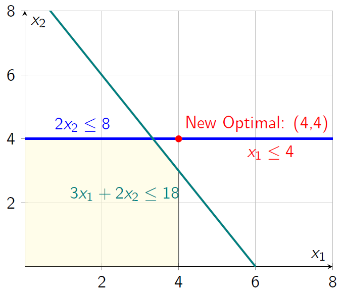
Sensitivity Analysis Example
Original Problem
Maximize \(Z
= 3x_1 + 5x_2\)
Subject to: \(\begin{cases}
x_1 \leq 4 \\
2x_2 \leq 12 \\
3x_1 + 2x_2 \leq 18 \\
x_1, x_2 \geq 0
\end{cases}\)
Change: Tighten \(2x_2
\leq 12\) to \(2x_2 \leq
8\).
Effect: New feasible region; optimal at \((4, 4)\), \(Z =
32\).
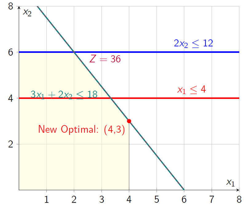
Sensitivity: Objective Function Change
Original
Problem:
Maximize \(Z = 3x_1 + 5x_2\)
Subject to: \(\begin{cases}
x_1 \leq 4 \\
2x_2 \leq 12 \\
3x_1 + 2x_2 \leq 18 \\
x_1, x_2 \geq 0
\end{cases}\)
Change: New objective \(Z
= 6x_1 + 4x_2\).
Effect: Slope changes; new optimal at \((4, 3)\), \(Z =
36\).
Case Study: Production Planning
Case Study: Furniture Manufacturing
Problem: A furniture factory produces chairs (\(x_1\)) and tables (\(x_2\)).
-
Objective: Maximize profit: \(Z = 20x_1 + 30x_2\).
-
Constraints: \(\begin{cases} 2x_1 + 5x_2 \leq 100 \quad (\text{wood, kg/day}) \\ 3x_1 + 2x_2 \leq 60 \quad (\text{labor, hours/day}) \\ x_1, x_2 \geq 0 \end{cases}\)
Steps:
-
Plot constraints to find the feasible region.
-
Identify corner points.
-
Evaluate \(Z\) at each corner point.
Case Study: Graphical Solution
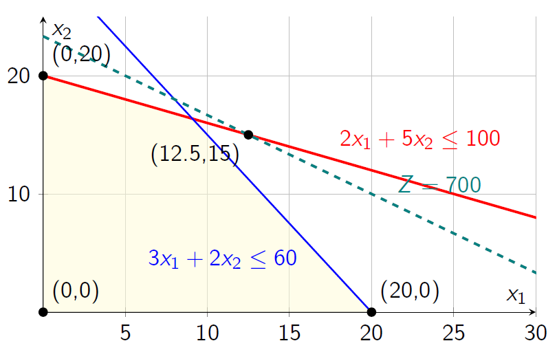
| Corner Point | Coordinates | Profit (Z) |
|---|---|---|
| (0, 0) | (0, 0) | 0 |
| (0, 20) | (0, 20) | 600 |
| (12.5, 15) | (12.5, 15) | 700 |
| (20, 0) | (20, 0) | 400 |
Conclusion
Optimal solution: \((x_1, x_2) = (12.5, 15)\), Profit = $700/day.
Limitations of Graphical Methods
-
Limited to 2 Variables: Impractical for problems with three or more decision variables.
-
Visualization Challenges: Complex constraints or large feasible regions are hard to plot accurately.
-
Scalability: Real-world engineering problems often involve thousands of variables.
-
Precision: Manual plotting may introduce errors in identifying corner points.
Solution
Algebraic methods like the Simplex Method handle higher-dimensional problems efficiently.
Summary
-
Graphical methods visualize constraints, feasible regions, and optimal solutions for 2D LP problems.
-
Corner-point method identifies the optimal solution by evaluating vertices.
-
Sensitivity analysis assesses the impact of changes in constraints or objective function.
-
Applications include production planning, resource allocation, and engineering design.
-
Limitations restrict graphical methods to small-scale problems.
Next Lecture
Simplex Method: Solving higher-dimensional LP problems algebraically.