Motivation and Context
Recall from Previous Lectures:
-
Necessary conditions for optimality (KKT conditions)
-
Sufficient conditions using Hessian matrix
-
Classification of critical points
Focus of this Topic:
-
How do we find these optimal points algorithmically?
-
Gradient descent: the foundational iterative method
Central Question
Given \(\min_{x \in \mathbb{R}^n} f(x)\) where \(f\) is smooth, how do we construct a sequence \(\{x_k\}\) that converges to \(x^*\)?
Why Gradient Descent?
Historical Context:
-
Cauchy (1847): First systematic use of steepest descent
-
Foundation for modern machine learning algorithms
-
Still the workhorse for large-scale optimization
Key Applications:
-
Machine Learning: Training neural networks
-
Statistics: Maximum likelihood estimation
-
Engineering: Parameter identification
-
Finance: Portfolio optimization
Why Start Here?
Understanding gradient descent is crucial for appreciating more sophisticated methods like Newton’s method and quasi-Newton approaches.
The Gradient Descent Algorithm
Key Insights:
-
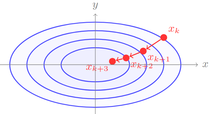
Gradient \(\nabla f(x)\) is perpendicular to level curves
-
Points in direction of steepest increase
-
Negative gradient gives steepest decrease
First-Order Taylor Expansion:
To minimize locally, choose \(d = -\alpha \nabla f(x)\)
Intuition: Following the Steepest Descent
-
At point \(x_k\), the gradient \(\nabla f(x_k)\) points in the direction of steepest ascent
-
To minimize \(f\), we move in the opposite direction: \(-\nabla f(x_k)\)
-
This is the direction of steepest descent
Definition: Gradient Descent
Starting from \(x_0 \in \mathbb{R}^n\), generate the sequence:
where \(\alpha_k > 0\) is the step size (learning rate) at iteration \(k\).
The method is also called steepest descent when exact line search is used.
Algorithm Statement
- Require Function \( f: \mathbb{R}^n \to \mathbb{R} \), initial point \( x_0 \), tolerance \( \epsilon > 0 \)
- \( k \leftarrow 0 \)
- while \( \|\nabla f(x_k)\| > \epsilon \) do
- Choose step size \( \alpha_k > 0 \)
- \( x_{k+1} \leftarrow x_k - \alpha_k \nabla f(x_k) \)
- \( k \leftarrow k + 1 \)
- Return \( x_k \)
Key Components:
-
Direction: \(d_k = -\nabla f(x_k)\) (steepest descent direction)
-
Step size: \(\alpha_k\) (how far to move)
-
Stopping criterion: \(\|\nabla f(x_k)\| \leq \epsilon\)
Alternative Stopping Criteria
Gradient Norm: \(\|\nabla f(x_k)\| \leq \epsilon_g\)
-
Most common and theoretically justified
-
Measures proximity to stationary point
Function Value Change: \(|f(x_k) - f(x_{k-1})| \leq \epsilon_f\)
-
Practical when function evaluation is expensive
-
May terminate prematurely in flat regions
Step Size: \(\|x_k - x_{k-1}\| \leq \epsilon_x\)
-
Useful when solution accuracy is more important than optimality
-
Can be misleading with small step sizes
Combined Criteria: Often use multiple conditions simultaneously
Step Size Selection
-
Fixed step size: \(\alpha_k = \alpha\) (constant)
-
Exact line search: \(\alpha_k = \arg\min_{\alpha > 0} f(x_k - \alpha \nabla f(x_k))\)
-
Inexact line search: Armijo rule, Wolfe conditions
-
Adaptive methods: AdaGrad, RMSprop, Adam (for ML)
Exact Line Search
At each iteration, solve the one-dimensional optimization problem:
Optimality condition: \(\phi'(\alpha_k) = 0\)
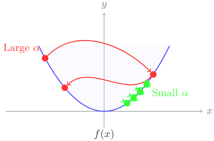
Step Size Selection: Trade-offs
Too Large Step Size:
-
May overshoot minimum
-
Can cause divergence
-
Oscillatory behavior
Too Small Step Size:
-
Very slow convergence
-
Many iterations needed
-
Computational inefficiency
Armijo Rule (Backtracking Line Search)
Idea: Start with a large step size and reduce until sufficient decrease condition is met.
Armijo Condition
Choose \(c_1 \in (0, 1)\) (typically \(c_1 = 10^{-4}\)). Accept \(\alpha_k\) if:
Backtracking Algorithm:
-
Start with \(\alpha = \alpha_0\) (e.g., \(\alpha_0 = 1\))
-
While Armijo condition fails: \(\alpha \leftarrow \rho \alpha\) (e.g., \(\rho = 0.5\))
-
Accept current \(\alpha\) as \(\alpha_k\)
Advantages: Guarantees sufficient decrease, adaptive to local function behavior
Wolfe Conditions
More sophisticated line search conditions:
Strong Wolfe Conditions
Given \(0 < c_1 < c_2 < 1\), accept \(\alpha_k\) if both:
Typical values: \(c_1 = 10^{-4}\), \(c_2 = 0.9\) (for Newton-type methods) or \(c_2 = 0.1\) (for conjugate gradient)
Benefits:
-
Ensures both sufficient decrease and sufficient progress
-
Prevents steps that are too small
-
Theoretical guarantees for many optimization algorithms
Convergence Analysis
Standard Assumptions:
-
\(f: \mathbb{R}^n \to \mathbb{R}\) is continuously differentiable
-
\(f\) is bounded below: \(f(x) \geq f_{\text{inf}} > -\infty\) for all \(x\)
-
\(\nabla f\) is Lipschitz continuous with constant \(L > 0\):
\[\|\nabla f(x) - \nabla f(y)\| \leq L \|x - y\|, \quad \forall x, y \in \mathbb{R}^n\]
Descent Property
If \(0 < \alpha_k < 2/L\), then gradient descent produces a monotone decreasing sequence:
Proof idea: Use Taylor expansion and Lipschitz condition to bound \(f(x_{k+1})\).
Descent lemma: Key Technical Result
Descent lemma
If \(\nabla f\) is \(L\)-Lipschitz continuous, then for any \(x, y \in \mathbb{R}^n\):
Application to Gradient Descent: Setting \(y = x_k - \alpha_k \nabla f(x_k)\):
If \(\alpha_k < 2/L\), then \(f(x_{k+1}) < f(x_k)\) (strict decrease).
Main Convergence Result
Theorem: Convergence of Gradient Descent
Under the Lipschitz assumption with constant \(L\), if we use fixed step size \(0 < \alpha \leq 1/L\), then:
Implications:
-
\(\|\nabla f(x_k)\| \to 0\) as \(k \to \infty\) (subsequence convergence)
-
Convergence rate: \(O(1/k)\) (sublinear)
-
To achieve \(\|\nabla f(x_k)\| \leq \epsilon\), need \(O(1/\epsilon^2)\) iterations
Note: This is a worst-case bound; actual performance often much better.
Stronger Convergence for Convex Functions
Theorem: Convex Case
If \(f\) is convex and satisfies the Lipschitz condition, then with \(\alpha \leq 1/L\):
Theorem: Strongly Convex Case
If \(f\) is \(\mu\)-strongly convex (\(\mu > 0\)) and \(L\)-smooth, then with \(\alpha = 2/(\mu + L)\):
This gives linear convergence with rate \(\rho = \frac{L - \mu}{L + \mu} < 1\).
Condition Number: \(\kappa = L/\mu\) determines convergence rate.
Understanding Condition Numbers
-
Theorem: For strongly convex function, condition number \(\kappa = L/\mu\)
-
Convergence rate: \(\rho = \frac{\kappa - 1}{\kappa + 1}\)
| \(\kappa\) | \(\rho\) | Convergence Quality |
|---|---|---|
| 1 | 0 | Excellent (one step) |
| 10 | 0.82 | Good |
| 100 | 0.98 | Poor |
| 1000 | 0.998 | Very poor |
Key Insight
Gradient descent struggles with ill-conditioned problems where \(\kappa \gg 1\). This motivates preconditioning and second-order methods.
Computational Aspects
Per iteration cost:
-
Gradient computation: \(O(n)\) for general functions
-
Vector operations: \(O(n)\)
-
Line search (if used): depends on function evaluation cost
Memory requirements:
-
Current point: \(x_k \in \mathbb{R}^n\)
-
Current gradient: \(\nabla f(x_k) \in \mathbb{R}^n\)
-
Total: \(O(n)\) memory
Advantages:
-
Simple implementation
-
Low memory requirements
-
Guaranteed descent (with proper step size)
-
Scales well to high dimensions
Implementation Considerations
Numerical Issues:
-
Gradient computation accuracy
-
Finite difference approximations
-
Round-off errors in step size selection
Practical Tips:
-
Monitor both gradient norm and function value
-
Use relative tolerances: \(\|\nabla f(x_k)\| \leq \epsilon_{\text{rel}} \cdot \|\nabla f(x_0)\|\)
-
Restart if progress stalls
-
Consider scaling/preconditioning for better conditioning
Debugging:
-
Verify gradient with finite differences
-
Check descent property: \(f(x_{k+1}) < f(x_k)\)
-
Plot convergence history
Limitations and Improvements
-
Slow convergence: Only \(O(1/k)\) rate in general
-
Condition number dependence: Poor performance when \(\kappa = L/\mu\) is large
-
No curvature information: Ignores second-order information
-
Sensitive to scaling: Performance depends on coordinate system
-
Local minima: Can get stuck in non-convex problems
Example: Poorly Conditioned Problem
Consider \(f(x_1, x_2) = \frac{1}{2}(x_1^2 + 100x_2^2)\)
-
Condition number: \(\kappa = 100\)
-
Gradient descent oscillates in narrow valley
-
Convergence rate: \(\rho = \frac{99}{101} \approx 0.98\) (very slow!)
Variants and Improvements
Momentum Methods:
-
Heavy ball method: \(x_{k+1} = x_k - \alpha \nabla f(x_k) + \beta(x_k - x_{k-1})\)
-
Nesterov acceleration: Look-ahead gradient evaluation
Adaptive Step Sizes:
-
AdaGrad: Accumulate squared gradients
-
RMSprop: Exponential moving average of squared gradients
-
Adam: Combine momentum and adaptive step sizes
Stochastic Variants:
-
Stochastic Gradient Descent (SGD)
-
Mini-batch methods
-
Variance reduction techniques (SVRG, SAGA)
Preview: Advanced Methods
Coming in next lectures:
-
Newton’s Method: Uses Hessian information
\[x_{k+1} = x_k - [\nabla^2 f(x_k)]^{-1} \nabla f(x_k)\] -
Quasi-Newton Methods: Approximate Hessian (BFGS, L-BFGS)
-
Conjugate Gradient: Exploits quadratic structure
-
Trust Region Methods: Adaptive step size selection
Key Insight
All these methods can be viewed as variants of the basic iteration:
Examples and Applications
-
Consider \(f(x) = \frac{1}{2} x^T A x - b^T x\) where \(A \succ 0\).
-
Gradient: \(\nabla f(x) = Ax - b\)
-
Optimal point: \(x^* = A^{-1} b\)
-
Gradient descent:
\[x_{k+1} = x_k - \alpha (Ax_k - b) = (I - \alpha A) x_k + \alpha b\] -
Error analysis: \(e_k = x_k - x^*\) satisfies \(e_{k+1} = (I - \alpha A) e_k\)
-
Convergence: Linear with rate \(\rho = \max\{|1 - \alpha \lambda_{\min}|, |1 - \alpha \lambda_{\max}|\}\)
-
Optimal step size: \(\alpha^* = \frac{2}{\lambda_{\min} + \lambda_{\max}}\) gives \(\rho^* = \frac{\kappa - 1}{\kappa + 1}\)
Example 2: Logistic Regression
Problem: Given data \((x_i, y_i)_{i=1}^m\) where \(y_i \in \{0,1\}\), minimize:
Gradient:
Properties:
-
\(f\) is convex (with regularization \(\lambda > 0\))
-
\(\nabla f\) is Lipschitz continuous
-
Gradient descent converges to global optimum
-
Widely used in machine learning
Example 3: Least Squares with Regularization
Problem: \(\min_x \frac{1}{2}\|Ax - b\|^2 + \frac{\lambda}{2}\|x\|^2\)
Gradient: \(\nabla f(x) = A^T(Ax - b) + \lambda x = (A^TA + \lambda I)x - A^Tb\)
Analysis:
-
Condition number: \(\kappa = \frac{\sigma_1^2 + \lambda}{\sigma_n^2 + \lambda}\) where \(\sigma_1 \geq \cdots \geq \sigma_n \geq 0\)
-
Regularization improves conditioning
-
For \(\lambda > 0\), always strongly convex
Practical considerations:
-
Can solve directly: \(x^* = (A^TA + \lambda I)^{-1} A^Tb\)
-
Gradient descent useful for very large problems
-
Iterative methods can be more efficient than direct solve
Practical Guidelines
Good Cases:
-
Large-scale problems (high dimensional)
-
When Hessian is expensive or unavailable
-
Smooth, well-conditioned problems
-
As a warm-start for other methods
-
Online/streaming optimization
Poor Cases:
-
Ill-conditioned problems
-
When high accuracy is needed quickly
-
Small problems where direct methods work
-
Highly non-convex functions with many local minima
Alternatives to Consider:
-
Newton’s method (if Hessian available)
-
Quasi-Newton methods (L-BFGS)
-
Conjugate gradient (for quadratic problems)
Parameter Tuning Guidelines
Step Size Selection:
-
Start with \(\alpha = 1\) and use backtracking
-
For quadratic functions: estimate condition number and use \(\alpha = 2/(L + \mu)\)
-
Monitor convergence: reduce if oscillating, increase if too slow
-
Consider adaptive methods for complex problems
Stopping Criteria:
-
Primary: \(\|\nabla f(x_k)\| \leq \epsilon_{abs} + \epsilon_{rel} \|\nabla f(x_0)\|\)
-
Secondary: Maximum iterations (prevent infinite loops)
-
Optional: Function value change or step size criteria
Implementation Tips:
-
Scale variables to similar ranges
-
Use good initial guess when possible
-
Monitor and plot convergence history
Common Pitfalls and Debugging
Common Issues:
-
Divergence: Step size too large, check \(\alpha < 2/L\)
-
Slow convergence: Problem is ill-conditioned, consider preconditioning
-
Oscillation: Step size too large or poor scaling
-
Premature termination: Tolerance too loose or wrong stopping criterion
Debugging Strategies:
-
Verify gradient implementation with finite differences
-
Check that function decreases at each iteration
-
Plot function value and gradient norm vs iteration
-
Test on simple quadratic functions first
-
Use line search to automatically adjust step size
Performance Monitoring:
-
Track: \(f(x_k)\), \(\|\nabla f(x_k)\|\), \(\|x_k - x_{k-1}\|\)
-
Look for: monotonic decrease, exponential convergence patterns
Summary and Outlook
Gradient Descent Fundamentals:
-
Simple, intuitive algorithm: move opposite to gradient direction
-
Guaranteed convergence under mild conditions
-
Sublinear convergence rate: \(O(1/k)\) in general case
Critical Factors:
-
Step size selection determines success/failure
-
Problem conditioning (\(\kappa = L/\mu\)) affects convergence speed
-
Proper scaling and initialization matter significantly
Practical Impact:
-
Foundation of modern machine learning optimization
-
Building block for more sophisticated methods
-
Still widely used for large-scale problems
Connection to Broader Optimization
Gradient Descent as Template:
| Method | Direction \(d_k\) | Properties |
|---|---|---|
| Gradient Descent | \(-\nabla f(x_k)\) | Simple, robust |
| Newton’s Method | \(-[\nabla^2 f(x_k)]^{-1}\nabla f(x_k)\) | Fast, quadratic convergence |
| Quasi-Newton | \(-B_k^{-1}\nabla f(x_k)\) | Balance speed/cost |
| Conjugate Gradient | Conjugate directions | Optimal for quadratic |
Unifying Principle: All methods choose direction \(d_k\) and step size \(\alpha_k\) to ensure convergence while optimizing computational efficiency.
Looking Forward
Next Topics:
-
Newton’s Method: Second-order information for faster convergence
-
Quasi-Newton Methods: Approximating Hessian efficiently
-
Constrained Optimization: Handling equality/inequality constraints
-
Stochastic Methods: Large-scale and noisy optimization
Advanced Topics:
-
Non-convex optimization landscapes
-
Parallel and distributed optimization
-
Online and streaming optimization
-
Robust optimization under uncertainty
Remember
Understanding gradient descent deeply provides the foundation for mastering all advanced optimization methods.
Next lecture: Newton’s Method and Second-Order Optimization