Why Study Duality?
Real-World Scenario
A factory manager asks: "Should I buy more raw materials or hire more workers to maximize profit?"
-
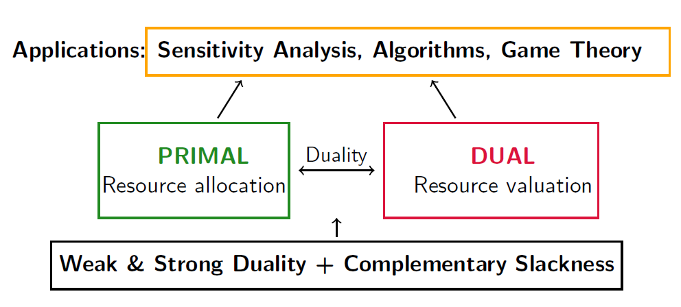
Primal Problem: How to allocate resources optimally?
-
Dual Problem: What is each resource worth?
-
Duality helps answer both questions simultaneously!
Learning Objectives
By the end of this lecture, you will:
-
Understand the concept and construction of dual problems
-
Apply duality theorems to solve optimization problems
-
Interpret shadow prices for decision-making
-
Use complementary slackness for solution verification
Fundamentals of Duality
For every linear programming problem (called the primal), there exists an associated optimization problem (called the dual) that provides insights into the original problem.
Primal Perspective
-
Question: How much to produce?
-
Goal: Maximize profit
-
Constraints: Limited resources
-
Variables: Production quantities
Dual Perspective
-
Question: What are resources worth?
-
Goal: Minimize resource cost
-
Constraints: Maintain profitability
-
Variables: Resource prices
Key Insight
The dual problem asks: "What should I pay for resources to make the original problem unprofitable?"
Standard Form: Primal-Dual Pair
Primal Problem (Max)
-
\(m\) constraints
-
\(n\) variables
-
Coefficient matrix: \(A\)
Dual Problem (Min)
-
\(n\) constraints
-
\(m\) variables
-
Coefficient matrix: \(A^T\)
Matrix Notation
Primal: \(\max \{\mathbf{c}^T\mathbf{x} : A\mathbf{x} \leq \mathbf{b}, \mathbf{x} \geq \mathbf{0}\}\) Dual: \(\min \{\mathbf{b}^T\mathbf{y} : A^T\mathbf{y} \geq \mathbf{c}, \mathbf{y} \geq \mathbf{0}\}\)
Constructing the Dual Problem
Transformation Rules
| Primal (Max) | Dual (Min) | ||
|---|---|---|---|
| Constraint | Variable | Variable | Constraint |
| \(\leq\) | \(\leftrightarrow\) \(\geq 0\) | \(\leftrightarrow\) | \(\geq\) |
| \(\geq\) | \(\leftrightarrow\) \(\leq 0\) | \(\leftrightarrow\) | \(\leq\) |
| \(=\) | \(\leftrightarrow\) unrestricted | \(\leftrightarrow\) | \(=\) |
Memory Aid
-
Primal constraints \(\leftrightarrow\) Dual variables
-
Primal variables \(\leftrightarrow\) Dual constraints
-
Primal objective coefficients \(\leftrightarrow\) Dual RHS
-
Primal RHS \(\leftrightarrow\) Dual objective coefficients
Construction Example
Given Primal Problem
Step-by-Step Construction
-
Variables: 3 primal constraints \(\Rightarrow\) 3 dual variables \((y_1, y_2, y_3)\)
-
Variable signs: \((\leq, \geq, =) \Rightarrow (y_1 \geq 0, y_2 \leq 0, y_3 \text{ unrestricted})\)
-
Constraints: 3 primal variables \(\Rightarrow\) 3 dual constraints
-
Constraint types: \((\geq 0, \geq 0, \text{unrestricted}) \Rightarrow (\geq, \geq, =)\)
Construction Example (Continued)
Resulting Dual Problem
Verification checkmark
-
Objective: MIN (opposite of MAX)
-
Coefficients: RHS becomes objective, objective becomes RHS
-
Matrix: \(A\) becomes \(A^T\)
-
Variables: Each constraint type determines corresponding variable sign
-
Constraints: Each variable type determines corresponding constraint type
Special Cases in Dual Construction
Case 1: Minimization Primal
Primal (Min):
Dual (Max):
Case 2: Mixed Constraints
-
Convert to standard form first
-
Apply transformation rules systematically
-
Handle unrestricted variables by substitution: \(x = x^+ - x^-\) where \(x^+, x^- \geq 0\)
Important Property
Dual of Dual = Primal: Taking the dual of the dual problem returns the original primal problem.
Economic Interpretation
Production Planning Context
-
Company: Produces products using limited resources
-
Competitor: Wants to buy all resources and shut down production
Company’s Problem
-
Decision: How much of each product to make?
-
Objective: Maximize profit
-
Constraints: Resource availability
-
Result: Optimal production plan
Competitor’s Problem
-
Decision: How much to pay for each resource?
-
Objective: Minimize total payment
-
Constraints: Make production unprofitable
-
Result: Fair resource prices
Key Insight
The dual solution gives the shadow prices - the marginal value of each resource!
Shadow Prices and Marginal Analysis
The shadow price \(y_i^*\) of resource \(i\) is the rate of change in the optimal objective value per unit increase in the availability of resource \(i\).
Interpretation
-
\(y_i^* = 2\) means: "One additional unit of resource \(i\) increases profit by $2"
-
\(y_i^* = 0\) means: "Resource \(i\) has surplus; additional units have no value"
-
Higher shadow price \(\Rightarrow\) More valuable resource
Business Applications
-
Resource Acquisition: Which resources should we prioritize buying?
-
Capacity Planning: Where should we invest in expansion?
-
Outsourcing Decisions: What’s the maximum we should pay for external resources?
-
Product Pricing: How does resource cost affect product profitability?
Fundamental Duality Theorems
Weak Duality
For any feasible solution \(\mathbf{x}\) to the primal and any feasible solution \(\mathbf{y}\) to the dual:
Proof Sketch
Consequences
-
Bounding: Dual provides upper bound on primal optimum
-
Infeasibility Detection: If \(\mathbf{c}^T\mathbf{x} > \mathbf{b}^T\mathbf{y}\), then one solution is infeasible
-
Unboundedness: If primal is unbounded \(\Rightarrow\) dual is infeasible
Strong Duality Theorem
If either the primal or dual problem has an optimal solution, then both have optimal solutions and their optimal objective values are equal:
Implications
-
Optimality Verification: If we find feasible solutions with equal objective values, both are optimal
-
Solution Methods: Can solve either problem to get both solutions
-
Economic Equilibrium: Total resource value equals total profit at optimum
Practical Use
-
Solve easier problem (fewer constraints)
-
Extract dual solution from primal tableau
-
Verify optimality using strong duality
-
Perform sensitivity analysis using shadow prices
Fundamental Theorem of LP Duality
For any primal-dual pair, exactly one of the following holds:
Four Possible Cases
-
Both optimal: Both problems have optimal solutions with equal objective values
-
Primal unbounded, dual infeasible: Primal \(\to +\infty\), dual has no feasible solution
-
Dual unbounded, primal infeasible: Dual \(\to -\infty\), primal has no feasible solution
-
Both infeasible: Neither problem has a feasible solution
Important Notes
-
Cases 2 and 3 cannot occur simultaneously (by weak duality)
-
Case 4 is rare but possible in practice
-
This theorem provides complete characterization of LP solution status
Practical Application
If primal solver reports "unbounded," we know dual is infeasible without solving it!
Complementary Slackness
Complementary Slackness
Let \((\mathbf{x}^*, \mathbf{y}^*)\) be optimal solutions to the primal-dual pair. Then:
Intuitive Meaning
-
Equation (1): If dual variable is positive \(\Rightarrow\) primal constraint is tight
-
Equation (2): If primal variable is positive \(\Rightarrow\) dual constraint is tight
-
Economic interpretation: No positive price for abundant resources
Complementary Slackness Table
| Primal Constraint | Dual Variable | Primal Variable | Dual Constraint |
|---|---|---|---|
| Slack \(> 0\) | \(y_i^* = 0\) | \(x_j^* = 0\) | Slack \(> 0\) |
| Slack \(= 0\) | \(y_i^* \geq 0\) | \(x_j^* \geq 0\) | Slack \(= 0\) |
Using Complementary Slackness
Given Information
Suppose we know the optimal primal solution: \(x_1^* = 4, x_2^* = 0, x_3^* = 3\)
And the constraint status:
-
Constraint 1: \(2x_1 + x_2 + x_3 \leq 11\) is tight (slack = 0)
-
Constraint 2: \(x_1 + 3x_2 + 2x_3 \leq 15\) has slack = 3
Applying Complementary Slackness
-
Since \(x_2^* = 0\), the corresponding dual constraint has slack \(> 0\)
-
Since constraint 1 is tight, \(y_1^* > 0\) (positive shadow price)
-
Since constraint 2 has slack \(> 0\), \(y_2^* = 0\) (zero shadow price)
-
Since \(x_1^*, x_3^* > 0\), their dual constraints are tight
Key Insight
Complementary slackness allows us to determine dual solution from primal solution without additional computation!
Complete Worked Example
Production Planning Problem
A company produces two products (A and B) using three resources (Labor, Materials, Machine time).
Primal Problem
-
\(x_1\): Units of product A
-
\(x_2\): Units of product B
-
Profit: $4/unit A, $5/unit B
Dual Problem
-
\(y_1\): Price per labor hour
-
\(y_2\): Price per material unit
-
Resources: 8 labor hours, 12 material units
Question
What are the optimal production quantities and resource values?
Solving the Primal Problem
Graphical Solution Method
-
Constraints:
-
\(x_1 + 2x_2 \leq 8\) (Labor constraint)
-
\(3x_1 + x_2 \leq 12\) (Material constraint)
-
\(x_1, x_2 \geq 0\) (Non-negativity)
-
-
Corner Points:
-
\((0,0)\): \(z = 0\)
-
\((0,4)\): \(z = 20\)
-
\((4,0)\): \(z = 16\)
-
Intersection: Solve \(\begin{cases} x_1 + 2x_2 = 8 \\ 3x_1 + x_2 = 12 \end{cases}\)
-
Finding Intersection Point
Optimal Solution: \((x_1^*, x_2^*) = \left(\frac{16}{5}, \frac{12}{5}\right)\), \(z^* = 4 \cdot \frac{16}{5} + 5 \cdot \frac{12}{5} = \frac{124}{5} = 24.8\)
Solving the Dual Problem
Using Complementary Slackness
From primal solution: Both constraints are binding (intersection point)
-
Labor constraint: \(\frac{16}{5} + 2 \cdot \frac{12}{5} = 8\) [\(\checkmark\)]
-
Material constraint: \(3 \cdot \frac{16}{5} + \frac{12}{5} = 12\) [\(\checkmark\)]
By complementary slackness: \(y_1^*, y_2^* > 0\), so dual constraints are binding:
Solving the System
Dual Solution: \((y_1^*, y_2^*) = \left(\frac{11}{5}, \frac{3}{5}\right)\), \(w^* = 8 \cdot \frac{11}{5} + 12 \cdot \frac{3}{5} = \frac{124}{5} = 24.8\)
Solution Verification and Interpretation
Verification of Duality Theorems
-
Strong Duality: \(z^* = w^* = 24.8\) \(\checkmark\)
-
Complementary Slackness:
-
Both primal constraints tight \(\Rightarrow y_1^*, y_2^* > 0\) \(\checkmark\)
-
Both primal variables positive \(\Rightarrow\) both dual constraints tight \(\checkmark\)
-
Economic Interpretation
-
Optimal Production: Produce 3.2 units of A and 2.4 units of B
-
Shadow Prices:
-
Labor: \(y_1^* = 2.2\) per hour - Each additional labor hour increases profit by $2.20
-
Materials: \(y_2^* = 0.6\) per unit - Each additional material unit increases profit by $0.60
-
-
Resource Valuation: Total resource value = $24.80
Management Insights
-
Labor is more valuable than materials (higher shadow price)
-
Should prioritize acquiring additional labor hours
-
Maximum willing to pay: $2.20/labor hour, $0.60/material unit
Advanced Applications
What-If Analysis Questions
-
What if we have 9 labor hours instead of 8?
-
What if material cost increases?
-
What if we introduce a new product?
-
What if resource availability changes significantly?
Using Shadow Prices for Quick Analysis
Scenario: One additional labor hour (9 instead of 8)
-
Predicted profit increase: \(y_1^* \times 1 = 2.2 \times 1 = \$2.20\)
-
New total profit: \(24.8 + 2.2 = \$27.00\)
-
Caution: Valid only within feasible range!
Range of Validity
Shadow prices are valid only for small changes. For large changes:
-
Resource constraints may become non-binding
-
New constraints may become binding
-
Need to re-solve the problem
Dual Simplex Method Introduction
When to Use Dual Simplex
-
Starting point: Dual feasible but primal infeasible
-
Common scenarios:
-
After adding new constraints to optimal solution
-
Problems with many \(\geq\) constraints
-
Sensitivity analysis when optimality is lost
-
Algorithm Overview
-
Check optimality: All RHS \(\geq 0\)? If yes, STOP (optimal found)
-
Select leaving variable: Choose most negative RHS
-
Select entering variable: Minimum ratio test on dual
-
Pivot: Update tableau and repeat
Key Advantage
Maintains dual feasibility throughout, making it ideal for sensitivity analysis and certain problem structures.
Connection to Game Theory
Two-Person Zero-Sum Games
-
Player 1’s Strategy Problem \(\leftrightarrow\) Player 2’s Dual Problem
-
Von Neumann’s Minimax Theorem = Strong Duality Theorem
-
Game Value = Optimal Objective Value
Player 1 (Row Player)
Player 2 (Column Player)
Economic Interpretation
Duality in games represents the balance between offensive and defensive strategies.
Network Flow Applications
Minimum Cost Flow Problem
-
Primal: Minimize shipping costs subject to supply/demand constraints
-
Dual: Node potentials (prices) that satisfy reduced cost conditions
Max Flow - Min Cut Theorem
-
Primal: Maximize flow from source to sink
-
Dual: Minimize cut capacity
-
Strong Duality: Maximum flow value = Minimum cut capacity
Transportation Problem Duality
-
Dual Variables: Supply prices \((u_i)\) and demand prices \((v_j)\)
-
Optimality Condition: \(u_i + v_j = c_{ij}\) for basic variables
-
MODI Method: Uses dual solution for optimality testing
Practical Benefit
Network duality enables efficient algorithms for large-scale logistics and transportation problems.
Computational Considerations
Decision Factors
-
Problem Size:
-
If \(m < n\) (fewer constraints than variables): Solve dual
-
If \(m > n\) (more constraints than variables): Solve primal
-
-
Structure:
-
Many \(\geq\) constraints: Convert and use dual simplex
-
Network structure: Use specialized algorithms
-
-
Sensitivity Analysis Needs:
-
If shadow prices are primary interest: Focus on dual
-
If variable values are primary: Focus on primal
-
Modern Practice
Most commercial solvers automatically:
-
Choose the most efficient formulation
-
Provide both primal and dual solutions
-
Generate sensitivity analysis reports
Interior Point Methods and Duality
Primal-Dual Interior Point Methods
-
Solve primal and dual simultaneously
-
Use duality gap as convergence measure
-
Maintain feasibility in both problems
Duality Gap
Advantages of Primal-Dual Approach
-
Natural Stopping Criterion: Stop when gap is sufficiently small
-
Numerical Stability: Better conditioning than simplex for some problems
-
Polynomial Complexity: Theoretical guarantee of efficient solution
-
Warm Starts: Easy to restart from previous solution
Applications
Particularly effective for large-scale problems in portfolio optimization, network design, and machine learning.
Common Mistakes and Best Practices
Mistake 1: Incorrect Dual Construction
-
Wrong: Forgetting to transpose coefficient matrix
-
Correct: Always use \(A^T\) in dual constraints
Mistake 2: Shadow Price Misinterpretation
-
Wrong: "Shadow price is valid for any change amount"
-
Correct: Shadow prices valid only for small changes within feasible range
Mistake 3: Complementary Slackness Application
-
Wrong: Assuming all variables/constraints are either zero or binding
-
Correct: Use logical deduction - if constraint has slack, dual variable is zero
Mistake 4: Sign Conventions
-
Wrong: Mixing up maximization and minimization forms
-
Correct: Always convert to standard form first, then apply rules systematically
Best Practices and Tips
Problem Setup
-
Standard Form First: Convert problem to standard form before constructing dual
-
Systematic Approach: Use transformation table consistently
-
Verify Construction: Check dimensions, signs, and correspondences
Solution Process
-
Choose Wisely: Solve the easier problem (fewer constraints/better structure)
-
Use Complementary Slackness: Extract dual solution from primal tableau
-
Verify Results: Check strong duality and complementary slackness conditions
Interpretation
-
Economic Context: Always relate mathematical results to business meaning
-
Sensitivity Bounds: Determine valid ranges for shadow price analysis
-
Decision Support: Use insights for resource allocation and strategic planning
Memory Aid: "DISC"
Dual construction, Interpretation, Sensitivity analysis, Complementary slackness
Practice and Extensions
Problem Setup
A furniture company makes chairs and tables using wood and labor:
Your Tasks
-
Construct the dual problem
-
Solve both primal and dual
-
Verify strong duality and complementary slackness
-
Interpret shadow prices economically
-
Analyze: "Should we buy 10 more wood units at $2 each?"
Hint
Use the systematic approach: standard form → dual construction → solution → verification → interpretation
Extensions and Advanced Topics
Beyond Basic Duality
-
Nonlinear Programming: Lagrangian duality, KKT conditions
-
Integer Programming: LP relaxation bounds, branch-and-bound
-
Stochastic Programming: Dual decomposition methods
-
Multi-objective Optimization: Pareto optimality and duality
Computational Advances
-
Parallel Computing: Distributed primal-dual algorithms
-
Machine Learning: Dual formulations in SVM, neural networks
-
Robust Optimization: Uncertainty and duality theory
-
Online Optimization: Dynamic pricing and resource allocation
Research Applications
-
Financial portfolio optimization
-
Supply chain network design
-
Energy market operations
-
Telecommunications network planning
Summary and Key Takeaways
Key Takeaways - The Big Picture
Conceptual Understanding
-
Duality is Everywhere: Every LP has a meaningful dual interpretation
-
Two Perspectives: Primal asks "how much?", dual asks "how valuable?"
-
Mathematical Elegance: Strong duality reveals deep optimization structure
-
Economic Insight: Shadow prices provide powerful decision-making tools
Practical Skills
-
Construction: Master systematic dual formulation
-
Solution: Use complementary slackness for efficient solving
-
Interpretation: Translate mathematical results to business insights
-
Analysis: Apply sensitivity analysis for robust decision-making
Success Formula
Theory + Practice + Interpretation = Mastery
Understanding duality theory + solving problems + economic interpretation = Complete expertise in linear programming
Final Thoughts and Next Steps
What Makes Duality Powerful?
-
Unified Framework: Connects optimization theory, economics, and computation
-
Practical Impact: Enables better business decisions through shadow price analysis
-
Algorithmic Foundation: Basis for most efficient LP solution methods
-
Theoretical Beauty: Reveals fundamental optimization principles
Recommended Practice
-
Work through more construction examples with mixed constraints
-
Practice complementary slackness on various problem types
-
Apply sensitivity analysis to real business scenarios
-
Explore computational tools that provide dual solutions
Looking Forward
Duality concepts extend far beyond linear programming:
-
Nonlinear optimization (Lagrangian duality)
-
Machine learning (kernel methods, neural networks)
-
Game theory and economics
-
Control theory and engineering applications
"In optimization, as in life, there are always two sides to every story."