Introduction
- Convex optimization: Optimizes convex functions over convex sets for guaranteed global solutions.
- Key concepts: Convex sets, functions, and optimality conditions ensure efficient algorithms.
- Applications: Critical in machine learning, control systems, and engineering design.
- Objective: This lecture explores convexity, conditions, and practical implications.
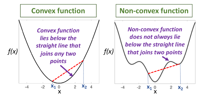
What is Convexity?
Convex Set
A set \( C \subseteq \mathbb{R}^n \) is convex if for any \( \mathbf{x}, \mathbf{y} \in C \), the line segment joining them lies in \( C \):
\[ \theta \mathbf{x} + (1-\theta) \mathbf{y} \in C \quad \forall \theta \in [0,1]. \]
Convex Function
A function \( f: C \to \mathbb{R} \) is convex if for all \( x, y \in C \) and \( \theta \in [0,1] \):
\[ f(\theta x + (1 - \theta)y) \leq \theta f(x) + (1 - \theta)f(y) \]
- Strictly convex: Inequality strict (\( < \)) for \( x \neq y \).
- Concave: \( -f \) is convex.
Why Study Convex Optimization?
- Global Optimality: Any local minimum is a global minimum.
- Efficient Algorithms: Solvable in polynomial time.
- Theory: KKT conditions are sufficient.
Key Insight: Convexity eliminates bad local minima, simplifying optimization.
Applications
- Linear/Quadratic Programming: Optimizing linear or quadratic objectives.
- Machine Learning: SVMs, regression models.
- Control Systems: Signal processing and design.
How to Test for Convexity?
First-Order Condition (Differentiable \( f \))
\( f \) is convex if:
\[ f(\mathbf{y}) \geq f(\mathbf{x}) + \nabla f(\mathbf{x})^T (\mathbf{y} - \mathbf{x}) \quad \forall \mathbf{x}, \mathbf{y} \in C. \]
(Function lies above its tangent hyperplane.)
Second-Order Condition (Twice Differentiable \( f \))
\( f \) is convex if its Hessian is positive semidefinite:
\[ \nabla^2 f(x) \succeq 0 \quad \forall x \in C. \]
For scalar functions: \( f''(x) \geq 0 \).
Example
- Scalar: \( f(x) = x^2 \), \( f''(x) = 2 > 0 \), convex.
- Multivariable: \( f(x,y) = x^2 + xy + y^2 \), Hessian \( \begin{pmatrix} 2 & 1 \\ 1 & 2 \end{pmatrix} \), eigenvalues \( 1, 3 \geq 0 \), convex.
Convex Optimization Problems
Standard Form
\[ \begin{aligned} \text{Minimize} \quad & f(\mathbf{x}) \\ \text{subject to} \quad & g_i(\mathbf{x}) \leq 0 \quad \text{(convex constraints)} \\ & h_j(\mathbf{x}) = 0 \quad \text{(affine constraints)}, \end{aligned} \]
where \( f \) and \( g_i \) are convex, \( h_j \) are affine.
Examples
- Linear Programming: \( f(\mathbf{x}) = \mathbf{c}^T \mathbf{x} \), \( g_i(\mathbf{x}) = \mathbf{a}_i^T \mathbf{x} - b_i \).
- Quadratic Programming: \( f(\mathbf{x}) = \frac{1}{2} \mathbf{x}^T Q \mathbf{x} + \mathbf{c}^T \mathbf{x} \), \( Q \succeq 0 \).
Non-Example
\( f(x) = x^3 \): Not convex (Hessian \( 6x \) not always \( \geq 0 \)).
Optimality Conditions
Theorem: Global Optimality
For convex \( f \), any \( \mathbf{x}^* \) with \( \nabla f(\mathbf{x}^*) = \mathbf{0} \) is a global minimum.
KKT for Convex Problems
- Necessary and Sufficient: If \( f \), \( g_i \) convex, \( h_j \) affine, and Slater’s condition holds, KKT conditions ensure optimality.
- No Duality Gap: Strong duality holds.
Slater’s Condition
Exists a strictly feasible point: \( g_i(\mathbf{x}) < 0 \) for all inequality constraints.
Practical Implications
- Reliability: Convex problems have tractable solutions.
- Algorithm Choice: Gradient descent, Newton’s method, interior-point methods with guaranteed convergence.
- Reformulation: Non-convex problems approximated as convex (e.g., relaxations in integer programming).
- Limitations: Not all problems are convex, but convexity is powerful when applicable.
Summary
- Convexity: Ensures global optimality and efficient algorithms.
- KKT Conditions: Necessary and sufficient for convex problems.
- Applications: Spans machine learning, engineering, and control systems.
- Next Steps: Explore numerical methods, engineering applications, and machine learning optimization.