Motivation and Background
Previously covered:
-
Gradient Descent: Simple but slow convergence
-
Newton’s Method: Fast but computationally expensive
Today’s Goal:
-
Bridge the gap between gradient descent and Newton’s method
-
Achieve superlinear convergence without computing Hessian
-
Handle large-scale problems efficiently
Key Insight
Use information from previous gradients to construct better search directions
Limitations of Previous Methods
Gradient Descent Issues:
-
Zigzag behavior near solution
-
Linear convergence rate
-
Poor performance on ill-conditioned problems
Newton’s Method Issues:
-
Requires Hessian computation: \(O(n^2)\) storage, \(O(n^3)\) factorization
-
May not be positive definite away from solution
-
Prohibitive for large-scale problems
The CG Solution
Achieve Newton-like performance using only gradient information!
Historical Development
Timeline of CG Development:
-
1952: Hestenes & Stiefel - Original CG method for linear systems
-
1964: Fletcher & Reeves - First nonlinear CG extension
-
1969: Polak & Ribière - Improved \(\beta\) formula
-
1976: Powell - Restart strategies and convergence analysis
-
1990s-2000s: Modern variants (Dai-Yuan, Liu-Storey, etc.)
Why CG Matters Today
-
Machine learning optimization (neural networks)
-
Large-scale scientific computing
-
Image processing and computer vision
-
Financial modeling and risk analysis
Mathematical Foundation
Consider minimizing a quadratic function:
where \(A\) is symmetric positive definite (SPD).
-
Gradient: \(\nabla f(x) = Ax - b\)
-
Solution: \(x^* = A^{-1}b\) (where \(\nabla f(x^*) = 0\))
-
Residual: \(r = b - Ax = -\nabla f(x)\)
Key Observation
Solving \(Ax = b\) is equivalent to minimizing the quadratic function
Concept of Conjugate Directions
For SPD matrix \(A\), directions \(\{p_0, p_1, \ldots, p_{k-1}\}\) are conjugate (or \(A\)-orthogonal) if:
Properties:
-
Generalize orthogonal directions
-
Form a basis for \(\mathbb{R}^n\)
-
Enable exact minimization in \(n\) steps

Why Conjugacy Works: Mathematical Intuition
Minimization in Subspaces: At iteration \(k\), CG finds the point \(x_k\) that minimizes \(f(x)\) over the affine subspace:
Expanding Subspaces:
-
\(k=0\): Minimize along line \(x_0 + \alpha p_0\)
-
\(k=1\): Minimize over plane \(x_0 + \alpha_0 p_0 + \alpha_1 p_1\)
-
\(k=n-1\): Minimize over entire space \(\mathbb{R}^n\)
Key Insight
Conjugacy ensures that minimizing in the new direction doesn’t "undo" progress made in previous directions
Geometric Interpretation: Why CG Works
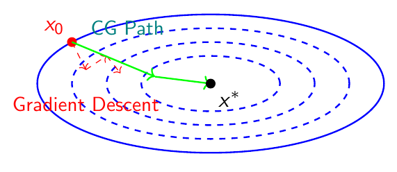
Key Insights:
-
CG avoids zigzag behavior
-
Each step uses optimal linear combination of gradients
-
Conjugate directions ensure no "backtracking"
-
Finite termination property
The Conjugate Gradient Algorithm
Algorithm: Conjugate Gradient Method
- Input: \( A \) (SPD), \( b \), initial guess \( x_0 \)
- \( r_0 = b - A x_0 \) (initial residual)
- \( p_0 = r_0 \) (initial search direction)
- For \( k = 0, 1, 2, \ldots \) until convergence:
- \( \alpha_k = \frac{r_k^T r_k}{p_k^T A p_k} \) (step size)
- \( x_{k+1} = x_k + \alpha_k p_k \) (update solution)
- \( r_{k+1} = r_k - \alpha_k A p_k \) (update residual)
- \( \beta_k = \frac{r_{k+1}^T r_{k+1}}{r_k^T r_k} \) (conjugacy parameter)
- \( p_{k+1} = r_{k+1} + \beta_k p_k \) (new search direction)
Understanding the CG Steps
-
Step Size \(\alpha_k\):
-
Exact line search along direction \(p_k\)
-
Minimizes \(f(x_k + \alpha p_k)\) with respect to \(\alpha\)
-
-
Residual Update:
-
\(r_{k+1} = b - Ax_{k+1} = -\nabla f(x_{k+1})\)
-
Can be computed efficiently: \(r_{k+1} = r_k - \alpha_k A p_k\)
-
-
Direction Update:
-
\(p_{k+1}\) combines new steepest descent direction \(r_{k+1}\) with previous direction \(p_k\)
-
\(\beta_k\) ensures conjugacy: \(p_{k+1}^T A p_i = 0\) for \(i \leq k\)
-
Derivation of CG Formulas
-
Step Size Derivation: To minimize \(f(x_k + \alpha p_k)\), set derivative w.r.t. \(\alpha\) to zero:
\[\begin{aligned} \frac{d}{d\alpha} f(x_k + \alpha p_k) &= \nabla f(x_k + \alpha p_k)^T p_k = 0 \\ (Ax_k + \alpha A p_k - b)^T p_k &= 0 \\ (-r_k + \alpha A p_k)^T p_k &= 0 \\ \alpha_k &= \frac{r_k^T p_k}{p_k^T A p_k} = \frac{r_k^T r_k}{p_k^T A p_k} \end{aligned}\] -
The last equality uses \(r_k^T p_j = 0\) for \(j < k\) (orthogonality property).
-
\(\beta_k\) Derivation: From conjugacy requirement \(p_{k+1}^T A p_k = 0\):
\[(r_{k+1} + \beta_k p_k)^T A p_k = 0 \Rightarrow \beta_k = -\frac{r_{k+1}^T A p_k}{p_k^T A p_k}\]
Key Properties of CG
Theorem: Fundamental CG Properties
For the CG algorithm applied to SPD system \(Ax = b\):
-
Conjugacy: \(p_i^T A p_j = 0\) for \(i \neq j\)
-
Orthogonality: \(r_i^T r_j = 0\) for \(i \neq j\)
-
Finite Termination: Exact solution in at most \(n\) steps
-
Optimality: \(x_k\) minimizes \(f(x)\) over \(x_0 + \text{span}\{p_0, \ldots, p_{k-1}\}\)
Krylov Subspace Connection
CG explores Krylov subspace: \(\mathcal{K}_k = \text{span}\{r_0, Ar_0, A^2r_0, \ldots, A^{k-1}r_0\}\)
Computational Complexity and Memory Requirements
Per Iteration Cost:
-
Matrix-vector product: \(O(n^2)\) for dense, \(O(\text{nnz})\) for sparse
-
Vector operations: \(O(n)\)
-
Total per iteration: Dominated by matrix-vector product
Memory Requirements:
-
Store vectors: \(x_k\), \(r_k\), \(p_k\) (3 vectors of size \(n\))
-
Matrix \(A\): \(O(n^2)\) for dense, \(O(\text{nnz})\) for sparse
-
Total: \(O(n^2)\) for dense problems, much less for sparse
Comparison with Direct Methods
-
Cholesky decomposition: \(O(n^3)\) time, \(O(n^2)\) space
-
CG: \(O(kn^2)\) time, \(O(n^2)\) space, where \(k \ll n\) typically
Numerical Example: 2D Quadratic
-
Consider: \(f(x) = \frac{1}{2}x^T \begin{pmatrix} 4 & 1 \\ 1 & 2 \end{pmatrix} x - \begin{pmatrix} 1 \\ 2 \end{pmatrix}^T x\)
-
Starting from \(x_0 = (0, 0)^T\):
Iteration 0:
-
\(r_0 = (1, 2)^T\)
-
\(p_0 = (1, 2)^T\)
-
\(\alpha_0 = \frac{5}{18}\)
-
\(x_1 = (\frac{5}{18}, \frac{10}{18})^T\)
Iteration 1:
-
\(r_1 = (\frac{4}{9}, -\frac{2}{9})^T\)
-
\(\beta_0 = \frac{4}{45}\)
-
\(p_1 = (\frac{4}{9} + \frac{4}{45}, -\frac{2}{9} + \frac{8}{45})^T\)
-
Exact solution reached!
Result
CG finds exact solution in 2 steps for 2D problem (as theory predicts)
Extension to Nonlinear Problems
-
For general nonlinear function \(f(x)\):
-
Replace residual \(r_k\) with negative gradient \(g_k = -\nabla f(x_k)\)
-
Use line search to find step size \(\alpha_k\)
-
Modify \(\beta_k\) formula (several variants exist)
-
Key Differences from Linear Case
-
No exact conjugacy (only approximate)
-
Requires line search for \(\alpha_k\)
-
May need periodic restarts
-
Multiple \(\beta_k\) formulas available
Nonlinear CG Algorithm
Algorithm: Nonlinear Conjugate Gradient
- Input: \( f(x) \), initial guess \( x_0 \)
- \( g_0 = \nabla f(x_0) \)
- \( p_0 = -g_0 \)
- For \( k = 0, 1, 2, \ldots \) until convergence:
- Find \( \alpha_k \) using line search to minimize \( f(x_k + \alpha p_k) \)
- \( x_{k+1} = x_k + \alpha_k p_k \)
- \( g_{k+1} = \nabla f(x_{k+1}) \)
- Compute \( \beta_k \) using chosen formula
- \( p_{k+1} = -g_{k+1} + \beta_k p_k \)
- If restart condition met:
- \( p_{k+1} = -g_{k+1} \) (restart with steepest descent)
Popular \(\beta_k\) Formulas
-
Fletcher-Reeves (1964):
\[\beta_k^{FR} = \frac{g_{k+1}^T g_{k+1}}{g_k^T g_k}\] -
Polak-Ribière (1969):
\[\beta_k^{PR} = \frac{g_{k+1}^T (g_{k+1} - g_k)}{g_k^T g_k}\] -
Hestenes-Stiefel (1952):
\[\beta_k^{HS} = \frac{g_{k+1}^T (g_{k+1} - g_k)}{p_k^T (g_{k+1} - g_k)}\] -
Dai-Yuan (1999):
\[\beta_k^{DY} = \frac{g_{k+1}^T g_{k+1}}{p_k^T (g_{k+1} - g_k)}\]
Comparison of \(\beta_k\) Formulas
-
Fletcher-Reeves:
-
Most robust, always well-defined
-
Can be slow on some problems
-
Reduces to linear CG for quadratics
-
-
Polak-Ribière:
-
Often performs better in practice
-
Automatically restarts when \(\beta_k < 0\)
-
More sensitive to line search accuracy
-
-
Hestenes-Stiefel & Dai-Yuan:
-
Good theoretical properties
-
Require careful implementation to avoid division by zero
-
Performance Comparison: \(\beta_k\) Formulas
| Property | FR | PR | HS | DY |
|---|---|---|---|---|
| Robustness | High | Medium | Medium | Medium |
| Practical Performance | Good | Excellent | Good | Good |
| Global Convergence | Yes | Yes* | Yes | Yes |
| Memory Required | Low | Low | Low | Low |
| Restart Frequency | High | Low | Medium | Low |
| Quadratic Reduction | Yes | No | No | No |
*PR requires exact line search for guaranteed convergence
Recommendation
Start with PR formula; switch to FR if convergence issues arise
Modern \(\beta_k\) Formulas and Hybrid Methods
Liu-Storey (1991):
Conjugate Descent (1987):
Hybrid Methods:
-
PR+: \(\beta_k = \max\{0, \beta_k^{PR}\}\) (automatic restart)
-
FR-PR: Switch between FR and PR based on performance
-
DY-HS: \(\beta_k = \max\{\beta_k^{DY}, \beta_k^{HS}\}\)
Recent Trend
Focus on self-adaptive methods that automatically adjust \(\beta_k\) based on problem characteristics
Line Search and Restart Strategies
For nonlinear CG, the line search must satisfy:
-
Sufficient Decrease: Armijo condition
\[f(x_k + \alpha_k p_k) \leq f(x_k) + c_1 \alpha_k g_k^T p_k\] -
Curvature Condition: Wolfe condition
\[g(x_k + \alpha_k p_k)^T p_k \geq c_2 g_k^T p_k\]where \(0 < c_1 < c_2 < 1\) (typically \(c_1 = 10^{-4}\), \(c_2 = 0.1\) for CG)
Strong Wolfe Conditions
For better performance, often use strong Wolfe conditions with \(|g(x_k + \alpha_k p_k)^T p_k| \leq c_2 |g_k^T p_k|\)
Restart Strategies
-
Why Restart?
-
Loss of conjugacy in nonlinear problems
-
Numerical errors accumulate
-
Search directions may become ineffective
-
-
Restart Criteria:
-
Periodic: Every \(n\) or \(n+1\) iterations
-
Gradient-based: When \(|g_{k+1}^T g_k| \geq \nu \|g_{k+1}\|^2\) (typically \(\nu = 0.1\))
-
Direction-based: When \(g_{k+1}^T p_k > 0\) (uphill direction)
-
Powell’s criterion: When \(\beta_k < 0\) for Polak-Ribière
-
-
Restart Action: Set \(p_{k+1} = -g_{k+1}\) (steepest descent direction)
Practical Line Search Implementation
-
Backtracking Line Search for CG:
- Set \( \alpha = \alpha_{\text{init}} \), \( \rho = 0.5 \), \( c = 10^{-4} \)
- While \( f(x_k + \alpha p_k) > f(x_k) + c \alpha g_k^T p_k \):
- \( \alpha = \rho \alpha \)
-
Initial Step Size Strategies:
-
\(\alpha_{\text{init}} = 1\) (Newton-like step)
-
\(\alpha_{\text{init}} = \frac{2(f_k - f_{k-1})}{g_k^T p_k}\) (based on function decrease)
-
\(\alpha_{\text{init}} = \frac{\alpha_{k-1} g_{k-1}^T p_{k-1}}{g_k^T p_k}\) (scaled previous step)
-
CG-Specific Consideration
CG typically requires less accurate line search than Newton methods, but more accurate than steepest descent
Termination Criteria for CG
Gradient-based Criteria:
-
Absolute: \(\|\nabla f(x_k)\| \leq \tau_1\)
-
Relative: \(\|\nabla f(x_k)\| \leq \tau_2 \|\nabla f(x_0)\|\)
-
Scaled: \(\|\nabla f(x_k)\| \leq \tau_3 (1 + |f(x_k)|)\)
Function-based Criteria:
-
Absolute change: \(|f(x_{k+1}) - f(x_k)| \leq \tau_4\)
-
Relative change: \(\frac{|f(x_{k+1}) - f(x_k)|}{1 + |f(x_k)|} \leq \tau_5\)
Step-based Criteria:
-
Step size: \(\alpha_k \|\mathbf{p}_k\| \leq \tau_6\)
-
Relative step: \(\frac{\|x_{k+1} - x_k\|}{\|x_k\| + 1} \leq \tau_7\)
Practical Values: \(\tau_1 = 10^{-6}\), \(\tau_2 = 10^{-6}\), \(\tau_3 = 10^{-8}\), \(\tau_4 = 10^{-12}\), \(\tau_5 = 10^{-8}\)
Recommendation
Use combination of gradient norm and relative function change for robust termination
Convergence Analysis
For quadratic function \(f(x) = \frac{1}{2}x^T A x - b^T x + c\) with condition number \(\kappa(A) = \frac{\lambda_{\max}}{\lambda_{\min}}\):
Theorem: CG Convergence Rate
The CG method satisfies:
where \(\|v\|_A = \sqrt{v^T A v}\) is the \(A\)-norm.
Key Insights:
-
Convergence depends on condition number \(\kappa(A)\)
-
Well-conditioned problems: \(\kappa(A) \approx 1 \Rightarrow\) fast convergence
-
Ill-conditioned problems: \(\kappa(A) \gg 1 \Rightarrow\) slow convergence
-
Superlinear convergence rate: better than gradient descent
Preconditioning
To improve convergence, solve equivalent system:
where \(M\) is a preconditioner chosen such that \(\kappa(M^{-1}A) \ll \kappa(A)\).
Popular Preconditioners:
-
Diagonal: \(M = \text{diag}(A)\) - Simple, limited effectiveness
-
Incomplete Cholesky: \(M = LL^T\) where \(L\) is sparse
-
Algebraic Multigrid: Excellent for elliptic PDEs
-
Domain Decomposition: For parallel computing
Trade-off
Better preconditioner \(\Rightarrow\) fewer CG iterations, but higher cost per iteration
Convergence for Nonlinear Problems
Global Convergence: Under suitable line search conditions, nonlinear CG methods converge to stationary points.
Convergence Rate:
-
Generally linear convergence
-
Can achieve superlinear convergence near solution for some variants
-
Rate depends on problem conditioning and \(\beta_k\) formula choice
Zoutendijk's Theorem
For CG with exact line search:
This implies \(\nabla f(x_k)^T p_k \to 0\), ensuring convergence.
Applications and Examples
Linear Systems:
-
Finite element analysis (structural mechanics, heat transfer)
-
Computational fluid dynamics
-
Image processing (deblurring, inpainting)
-
Graph algorithms (PageRank, spectral clustering)
Nonlinear Optimization:
-
Neural network training (especially for large networks)
-
Machine learning (logistic regression, SVM)
-
Parameter estimation in scientific models
-
Portfolio optimization in finance
-
Shape optimization in engineering design
Why CG for These Problems?
-
Low memory requirements
-
Good performance on large-scale problems
-
No need for Hessian computation
Case Study: Training Neural Networks
Problem Setup:
-
Minimize loss function \(L(\theta) = \sum_{i=1}^m \ell(h_{\theta}(x_i), y_i)\)
-
\(\theta\) are network parameters (potentially millions)
-
Gradient \(\nabla L(\theta)\) computed via backpropagation
CG vs Other Methods:
CG Advantages:
-
Memory efficient
-
No hyperparameter tuning
-
Good convergence properties
-
Handles non-convexity well
SGD/Adam Advantages:
-
Stochastic updates
-
Better for non-convex landscapes
-
More robust to noise
-
Established in practice
Hybrid Approaches: Use CG for fine-tuning after initial SGD training
Numerical Experiments: Performance Comparison
Test Problem: Extended Rosenbrock function in \(\mathbb{R}^{1000}\)
| Method | Iterations | Function Evals | Final Error |
|---|---|---|---|
| Steepest Descent | 50000+ | 100000+ | \(10^{-3}\) |
| CG (FR) | 2847 | 5694 | \(10^{-6}\) |
| CG (PR) | 1923 | 4156 | \(10^{-6}\) |
| BFGS | 1456 | 2912 | \(10^{-6}\) |
| Newton | 234 | 468 | \(10^{-6}\) |
Observations: CG significantly outperforms steepest descent, competitive with quasi-Newton methods
Advanced Topics
Idea: Use CG to approximately solve Newton equation \(\nabla^2 f(x_k) p = -\nabla f(x_k)\)
Algorithm:
-
Apply CG to Newton system (without forming Hessian)
-
Use Hessian-vector products: \(\nabla^2 f(x_k) v\)
-
Stop CG early when sufficient accuracy reached
Hessian-Vector Product Computation:
Advantages:
-
Newton-like convergence without storing Hessian
-
Adaptive accuracy (inner CG iterations)
-
Suitable for large-scale problems
Constrained Optimization: CG in Projected Gradient
-
Problem: Minimize \(f(x)\) subject to \(x \in \mathcal{C}\) (convex constraint set)
-
Projected CG Algorithm:
- \( x_0 \in \mathcal{C} \), \( g_0 = \nabla f(x_0) \), \( p_0 = -P_{\mathcal{C}}(x_0, g_0) \)
- For \( k = 0, 1, 2, \ldots \):
- Find \( \alpha_k \) such that \( x_k + \alpha_k p_k \in \mathcal{C} \)
- \( x_{k+1} = x_k + \alpha_k p_k \)
- \( g_{k+1} = \nabla f(x_{k+1}) \)
- Compute \( \beta_k \) and update \( p_{k+1} \)
- Project: \( p_{k+1} = P_{\mathcal{C}}(x_{k+1}, p_{k+1}) \)
where \(P_{\mathcal{C}}(x, d)\) projects direction \(d\) onto feasible cone at \(x\).
-
Applications: Box constraints, linear constraints, semidefinite programming
Parallel Implementation of CG
Main Computational Kernels:
-
Matrix-vector products: \(Ap_k\)
-
Vector dot products: \(r_k^T r_k\), \(p_k^T A p_k\)
-
Vector updates: \(x_{k+1} = x_k + \alpha_k p_k\)
Parallelization Strategies:
-
Data Parallelism: Distribute vector elements across processors
-
Matrix Parallelism: Distribute matrix rows/columns
-
Pipeline Parallelism: Overlap computation and communication
Challenges:
-
Global reductions (dot products) require communication
-
Load balancing for sparse matrices
-
Memory bandwidth limitations
Performance
CG achieves good parallel efficiency on modern HPC systems (80-90% typical)
Implementation Guidelines
Numerical Stability:
-
Use double precision arithmetic
-
Monitor for breakdown: \(p_k^T A p_k \approx 0\)
-
Implement robust dot product computation
-
Check for infinite/NaN values
Performance Optimization:
-
Efficient sparse matrix-vector multiplication
-
Memory access patterns (cache optimization)
-
Vectorization of operations
-
Minimize memory allocations
Robustness:
-
Implement multiple \(\beta_k\) formulas
-
Automatic restart strategies
-
Adaptive line search parameters
-
Graceful handling of edge cases
Common Implementation Pitfalls
Numerical Issues:
-
Loss of orthogonality due to finite precision
-
Indefinite preconditioners
-
Poor line search implementation
Algorithmic Issues:
-
Wrong \(\beta_k\) formula for problem type
-
Inadequate restart frequency
-
Incorrect termination criteria
Performance Issues:
-
Inefficient matrix storage format
-
Poor memory layout
-
Unnecessary function evaluations
Debug Strategy
Monitor convergence history, gradient norms, and search direction quality
Software Libraries and Tools
High-Quality CG Implementations:
-
MATLAB:
pcgfunction for linear systems -
SciPy:
scipy.optimize.minimizewith CG method -
PETSc: Parallel CG for large-scale linear systems
-
Eigen: C++ template library with CG solver
-
CG_DESCENT: Specialized nonlinear CG implementation
Machine Learning Frameworks:
-
TensorFlow/PyTorch: CG optimizers for neural networks
-
Optax (JAX): Modern optimization library with CG
Choosing Implementation:
-
Research/prototyping: MATLAB/Python
-
Production/performance: C++/Fortran
-
Large-scale parallel: PETSc/Trilinos
Summary and Future Directions
CG Method Strengths:
-
Bridges gap between gradient descent and Newton’s method
-
Low memory requirements: \(O(n)\) storage
-
Superlinear convergence for well-conditioned problems
-
No Hessian computation required
-
Finite termination for quadratic problems
When to Use CG:
-
Large-scale optimization problems
-
Sparse linear systems
-
Problems where Hessian is expensive/unavailable
-
When memory is limited
When NOT to Use CG:
-
Small problems (Newton’s method preferred)
-
Highly ill-conditioned problems without preconditioning
-
Problems with cheap, accurate Hessian
Current Research Directions
Adaptive Methods:
-
Self-tuning \(\beta_k\) formulas
-
Automatic restart strategies
-
Problem-specific parameter selection
Machine Learning Applications:
-
CG for deep learning optimization
-
Stochastic variants of CG
-
CG in reinforcement learning
High-Performance Computing:
-
GPU acceleration of CG
-
Communication-avoiding algorithms
-
Fault-tolerant implementations
Theoretical Advances:
-
Convergence analysis for non-convex problems
-
Randomized and quantum variants
-
CG for structured optimization problems
Next Steps in Your Learning Journey
Immediate Next Steps:
-
Implement basic CG algorithm for quadratic functions
-
Experiment with different \(\beta_k\) formulas
-
Test on various optimization problems
Advanced Topics to Explore:
-
Preconditioning techniques
-
Truncated Newton methods
-
Constrained optimization with CG
-
Parallel implementation